Time Series and Prometheus
1. What is Time Series
In mathematics, a time series is a series of data points indexed (or listed or graphed) in time order. Most commonly, a time series is a sequence taken at successive equally spaced points in time. Thus it is a sequence of discrete-time data.
| Time | Value |
|---|---|
09:00 |
24°C |
10:00 |
26°C |
11:00 |
27°C |
Time series are powerful. They help you understand the past by letting you analyze the state of the system at any point in time. Time series could tell you that the server crashed moments after the free disk space went down to zero.
Time series analysis comprises methods for analyzing time series data in order to extract meaningful statistics and other characteristics of the data. Time series forecasting is the use of a model to predict future values based on previously observed values.
1.1. Name and Labels
The common case is issuing a single query for a measurement with one or more additional properties as dimensions. For example, querying a temperature measurement along with a location property. In this case, multiple series are returned back from that single query and each series has unique location as a dimension.
Every time series is uniquely identified by its metric name and optional key-value pairs for identifying dimensions called labels.
Example labels could be {location=us} or {country=us,state=ma,city=boston}. Within a set of time series, the combination of its name and labels identifies each series.
Given a metric name and a set of labels, time series are frequently identified using this notation:
<metric name>{<label name>=<label value>, ...}For example, a time series with the metric name temperature and the labels country=us, state=ma and city=boston could be written like this:
temperature{country=us,state=ma,city=boston}For example, temperature {country=us,state=ma,city=boston} could identify the series of temperature values for the city of Boston in the US.
In table databases such SQL, these dimensions are generally the GROUP BY parameters of a query.
For example, consider a query like:
SELECT BUCKET(StartTime, 1h), AVG(Temperature) AS Temp, Location FROM T
  GROUP BY BUCKET(StartTime, 1h), Location
  ORDER BY time asc
This query would return a table with three columns with data types time, number, and string respectively:
| StartTime | Temp | Location |
|---|---|---|
09:00 |
24 |
LGA |
09:00 |
20 |
BOS |
10:00 |
26 |
LGA |
10:00 |
22 |
BOS |
1.2. Aggregation
Combining a collection of measurements is called aggregation. There are several ways to aggregate time series data. Here are some common ones:
-
Average returns the sum of all values divided by the total number of values.
-
Min and Max return the smallest and largest value in the collection.
-
Sum returns the sum of all values in the collection.
-
Count returns the number of values in the collection.
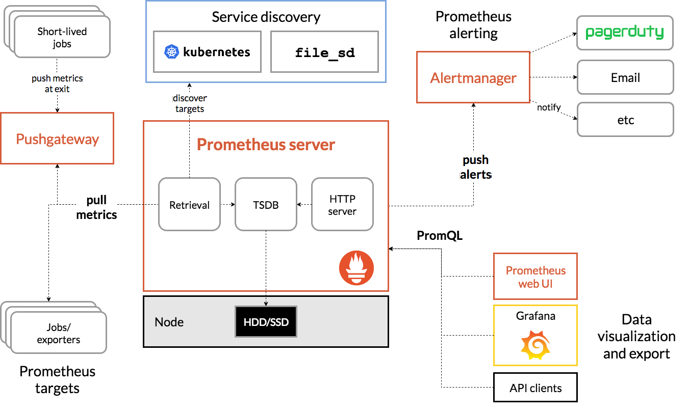
2. What is Prometheus?
Prometheus is an open-source systems monitoring and alerting toolkit originally built at SoundCloud. Prometheus joined the Cloud Native Computing Foundation in 2016 as the second hosted project, after Kubernetes.
Prometheus collects and stores its metrics as time series data, i.e. metrics information is stored with the timestamp at which it was recorded, alongside optional key-value pairs called labels.
2.1. Metric Types
The Prometheus offer four core metric types: counter, gauge, histogram, summary.
-
Counter
A counter is a cumulative metric that represents a single monotonically increasing counter whose value can only increase or be reset to zero on restart. For example, you can use a counter to represent the number of requests served, tasks completed, or errors.
Do not use a counter to expose a value that can decrease. For example, do not use a counter for the number of currently running processes; instead use a gauge.
-
Gauge
A gauge is a metric that represents a single numerical value that can arbitrarily go up and down.
Gauges are typically used for measured values like temperatures or current memory usage, but also "counts" that can go up and down, like the number of concurrent requests.
-
Histogram
A histogram samples observations (usually things like request durations or response sizes) and counts them in configurable buckets. It also provides a sum of all observed values.
A histogram with a base metric name of
<basename>exposes multiple time series during a scrape:-
cumulative counters for the observation buckets, exposed as
<basename>_bucket{le="<upper inclusive bound>"} -
the total sum of all observed values, exposed as
<basename>_sum -
the count of events that have been observed, exposed as
<basename>_count(identical to<basename>_bucket{le="+Inf"}above)
-
-
Summary
Similar to a histogram, a summary samples observations (usually things like request durations and response sizes). While it also provides a total count of observations and a sum of all observed values, it calculates configurable quantiles over a sliding time window.
A summary with a base metric name of
<basename>exposes multiple time series during a scrape:-
streaming φ-quantiles (0 ≤ φ ≤ 1) of observed events, exposed as
<basename>{quantile="<φ>"} -
the total sum of all observed values, exposed as
<basename>_sum -
the count of events that have been observed, exposed as
<basename>_count
-
2.2. PromQL
Prometheus provides a functional query language called PromQL (Prometheus Query Language) that lets the user select and aggregate time series data in real time.
In Prometheus’s expression language, an expression or sub-expression can evaluate to one of four types:
-
Instant vector - a set of time series containing a single sample for each time series, all sharing the same timestamp
-
Range vector - a set of time series containing a range of data points over time for each time series
-
Scalar - a simple numeric floating point value
-
String - a simple string value; currently unused
2.2.1. Instant vector selectors
Instant vector selectors allow the selection of a set of time series and a single sample value for each at a given timestamp (instant): in the simplest form, only a metric name is specified. This results in an instant vector containing elements for all time series that have this metric name.
This example selects all time series that have the http_requests_total metric name:
http_requests_totalIt is possible to filter these time series further by appending a comma separated list of label matchers in curly braces ({}).
This example selects only those time series with the http_requests_total metric name that also have the job label set to prometheus and their group label set to canary:
http_requests_total{job="prometheus",group="canary"}It is also possible to negatively match a label value, or to match label values against regular expressions. The following label matching operators exist:
-
=: Select labels that are exactly equal to the provided string.
-
!=: Select labels that are not equal to the provided string.
-
=~: Select labels that regex-match the provided string.
-
!~: Select labels that do not regex-match the provided string.
For example, this selects all http_requests_total time series for staging, testing, and development environments and HTTP methods other than GET.
http_requests_total{environment=~"staging|testing|development",method!="GET"}Label matchers can also be applied to metric names by matching against the internal name label. For example, the expression http_requests_total is equivalent to {name="http_requests_total"}.
2.2.2. Range Vector Selectors
Range vector literals work like instant vector literals, except that they select a range of samples back from the current instant. Syntactically, a time duration is appended in square brackets ([]) at the end of a vector selector to specify how far back in time values should be fetched for each resulting range vector element.
In this example, we select all the values we have recorded within the last 5 minutes for all time series that have the metric name http_requests_total and a job label set to prometheus:
http_requests_total{job="prometheus"}[5m]2.3. Federation
Federation allows a Prometheus server to scrape selected time series from another Prometheus server.
On any given Prometheus server, the /federate endpoint allows retrieving the current value for a selected set of time series in that server. At least one match[] URL parameter must be specified to select the series to expose. Each match[] argument needs to specify an instant vector selector like up or {job="api-server"}. If multiple match[] parameters are provided, the union of all matched series is selected.
$ curl -XGET -G \
    --data-urlencode 'match[]={job="kubernetes-endpoints", namespace="ingress-nginx"}' \
    https://prometheus.local.io/federate
To federate metrics from one server to another, configure your destination Prometheus server to scrape from the /federate endpoint of a source server, while also enabling the honor_labels scrape option and passing in the desired match[] parameters.
2.4. HTTP API
The following endpoint returns an overview of the current state of the Prometheus target discovery:
GET /api/v1/targetsBoth the active and dropped targets are part of the response by default. labels represents the label set after relabelling has occurred. discoveredLabels represent the unmodified labels retrieved during service discovery before relabelling has occurred.
The state query parameter allows the caller to filter by active or dropped targets, (e.g., state=active, state=dropped, state=any). Note that an empty array is still returned for targets that are filtered out. Other values are ignored.
$ curl -s localhost:9090/api/v1/targets | jq
{
  "status": "success",
  "data": {
    "activeTargets": [
      {
        "discoveredLabels": {
          "__address__": "localhost:9090",
          "__metrics_path__": "/metrics",
          "__scheme__": "http",
          "__scrape_interval__": "15s",
          "__scrape_timeout__": "10s",
          "job": "prometheus"
        },
        "labels": {
          "instance": "localhost:9090",
          "job": "prometheus"
        },
        "scrapePool": "prometheus",
        "scrapeUrl": "http://localhost:9090/metrics",
        "globalUrl": "http://node-01:9090/metrics",
        "lastError": "",
        "lastScrape": "2021-12-09T14:35:32.832227246+08:00",
        "lastScrapeDuration": 0.004144766,
        "health": "up",
        "scrapeInterval": "15s",
        "scrapeTimeout": "10s"
      }
    ],
    "droppedTargets": []
  }
}
2.5. Local Storage
Prometheus includes a local on-disk time series database, but also optionally integrates with remote storage systems.
Prometheus’s local time series database stores data in a custom, highly efficient format on local storage.
-
Ingested samples are grouped into blocks of two hours.
-
Each two-hour block consists of a directory containing a chunks subdirectory containing all the time series samples for that window of time, a metadata file, and an index file (which indexes metric names and labels to time series in the chunks directory).
-
The samples in the chunks directory are grouped together into one or more segment files of up to 512MB each by default.
-
When series are deleted via the API, deletion records are stored in separate tombstone files (instead of deleting the data immediately from the chunk segments).
-
The current block for incoming samples is kept in memory and is not fully persisted.
-
It is secured against crashes by a write-ahead log (WAL) that can be replayed when the Prometheus server restarts.
-
Write-ahead log files are stored in the wal directory in 128MB segments.
-
These files contain raw data that has not yet been compacted; thus they are significantly larger than regular block files.
-
Prometheus will retain a minimum of three write-ahead log files.
-
High-traffic servers may retain more than three WAL files in order to keep at least two hours of raw data.
A Prometheus server’s data directory looks something like this:
./data
├── 01BKGV7JBM69T2G1BGBGM6KB12
│   └── meta.json
├── 01BKGTZQ1SYQJTR4PB43C8PD98
│   ├── chunks
│   │   └── 000001
│   ├── tombstones
│   ├── index
│   └── meta.json
├── 01BKGTZQ1HHWHV8FBJXW1Y3W0K
│   └── meta.json
├── 01BKGV7JC0RY8A6MACW02A2PJD
│   ├── chunks
│   │   └── 000001
│   ├── tombstones
│   ├── index
│   └── meta.json
├── chunks_head
│   └── 000001
└── wal
    ├── 000000002
    └── checkpoint.00000001
└── 00000000|
Write-ahead logging (WAL)
In computer science, write-ahead logging (WAL) is a family of techniques for providing atomicity and durability (two of the ACID properties) in database systems. The changes are first recorded in the log, which must be written to stable storage, before the changes are written to the database. In a system using WAL, all modifications are written to a log before they are applied. Usually both redo and undo information is stored in the log. The purpose of this can be illustrated by an example. Imagine a program that is in the middle of performing some operation when the machine it is running on loses power. Upon restart, that program might need to know whether the operation it was performing succeeded, succeeded partially, or failed. If a write-ahead log is used, the program can check this log and compare what it was supposed to be doing when it unexpectedly lost power to what was actually done. On the basis of this comparison, the program could decide to undo what it had started, complete what it had started, or keep things as they are. WAL allows updates of a database to be done in-place. Another way to implement atomic updates is with shadow paging, which is not in-place. The main advantage of doing updates in-place is that it reduces the need to modify indexes and block lists. ARIES is a popular algorithm in the WAL family. Modern file systems typically use a variant of WAL for at least file system metadata; this is called journaling. |