Designing Data-Intensive Applications: B-Trees and LSM-Trees
Consider the world’s simplest database, implemented as two Bash functions:
#!/bin/bash

db_set () {
    echo "$1,$2" >> database
}

db_get () {
    grep "^$1," database | sed -e "s/^$1,//" | tail -n 1
}
These two functions implement a key-value store. You can call db_set key value, which will store key and value in the database. The key and value can be (almost) anything you like—for example, the value could be a JSON document. You can then call db_get key, which looks up the most recent value associated with that particular key and returns it.
And it works:
$ db_set 123456 '{"name":"London","attractions":["Big Ben","London Eye"]}'
$ db_set 42 '{"name":"San Francisco","attractions":["Golden Gate Bridge"]}'
$ db_get 42
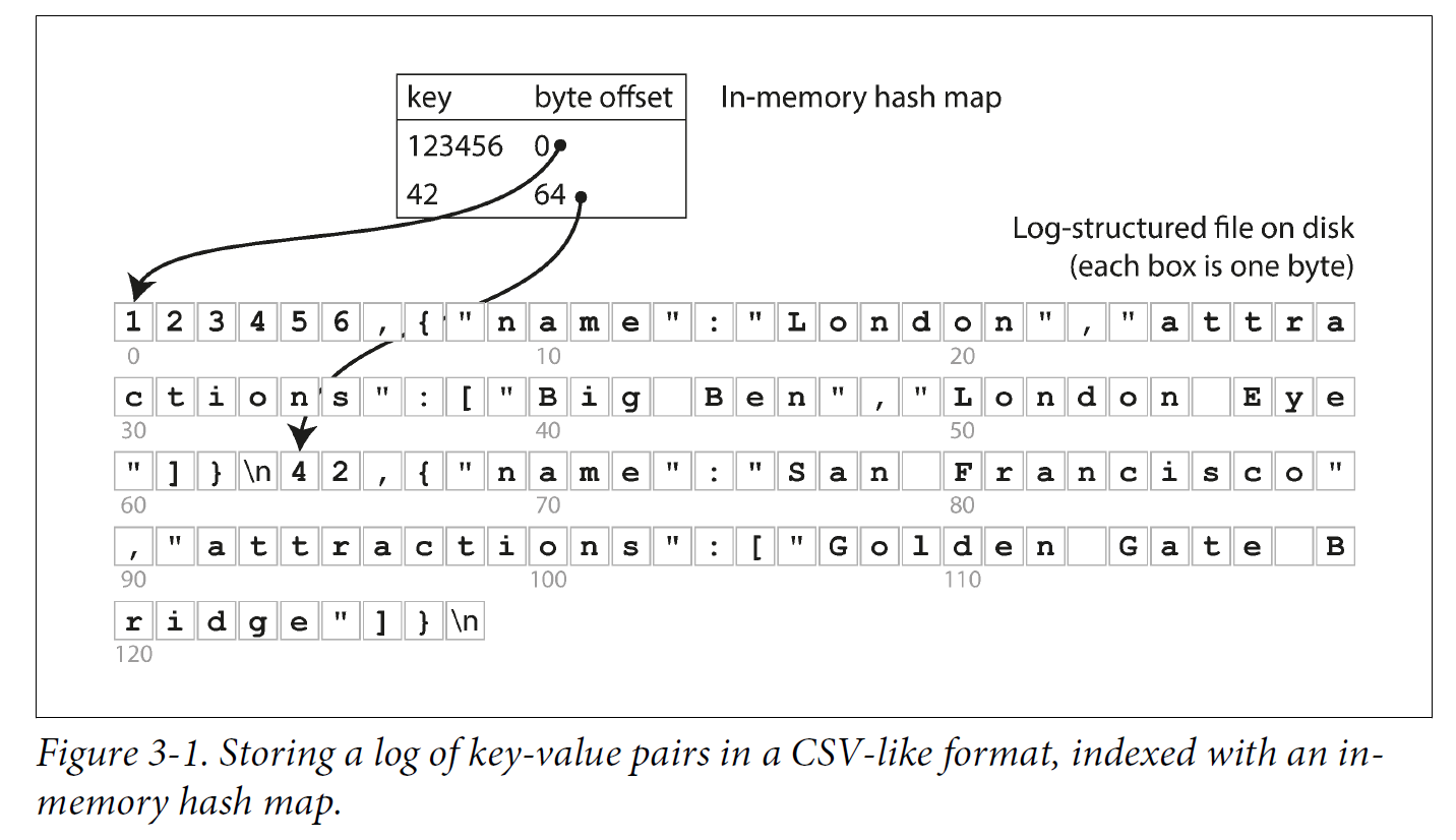
{"name":"San Francisco","attractions":["Golden Gate Bridge"]}The underlying storage format is very simple: a text file where each line contains a key-value pair, separated by a comma (roughly like a CSV file, ignoring escaping issues). Every call to db_set appends to the end of the file, so if you update a key several times, the old versions of the value are not overwritten—you need to look at the last occurrence of a key in a file to find the latest value (hence the tail -n 1 in db_get):
$ db_set 42 '{"name":"San Francisco","attractions":["Exploratorium"]}'

$ db_get 42
{"name":"San Francisco","attractions":["Exploratorium"]}

$ cat database
123456,{"name":"London","attractions":["Big Ben","London Eye"]}
42,{"name":"San Francisco","attractions":["Golden Gate Bridge"]}
42,{"name":"San Francisco","attractions":["Exploratorium"]}
Our db_set function actually has pretty good performance for something that is so simple, because appending to a file is generally very efficient. Similarly to what db_set does, many databases internally use a log, which is an append-only data file.
On the other hand, our db_get function has terrible performance if you have a large number of records in your database. Every time you want to look up a key, db_get has to scan the entire database file from beginning to end, looking for occurrences of the key. In algorithmic terms, the cost of a lookup is O(n): if you double the number of records n in your database, a lookup takes twice as long. That’s not good.
In order to efficiently find the value for a particular key in the database, we need a different data structure: an index. An index is an additional structure that is derived from the primary data. Many databases allow you to add and remove indexes, and this doesn’t affect the contents of the database; it only affects the performance of queries. Maintaining additional structures incurs overhead, especially on writes. For writes, it’s hard to beat the performance of simply appending to a file, because that’s the simplest possible write operation. Any kind of index usually slows down writes, because the index also needs to be updated every time data is written.
1. Hash Indexes
Let’s start with indexes for key-value data. This is not the only kind of data you can index, but it’s very common, and it’s a useful building block for more complex indexes.
Key-value stores are quite similar to the dictionary type that you can find in most programming languages, and which is usually implemented as a hash map (hash table). Since we already have hash maps for our in-memory data structures, why not use them to index our data on disk?
Let’s say our data storage consists only of appending to a file, as in the preceding example. Then the simplest possible indexing strategy is this: keep an in-memory hash map where every key is mapped to a byte offset in the data file—the location at which the value can be found.
-
Whenever you append a new key-value pair to the file, you also update the hash map to reflect the offset of the data you just wrote (this works both for inserting new keys and for updating existing keys).
-
When you want to look up a value, use the hash map to find the offset in the data file, seek to that location, and read the value.
As described so far, we only ever append to a file—so how do we avoid eventually running out of disk space?
-
A good solution is to break the log into segments of a certain size by closing a segment file when it reaches a certain size, and making subsequent writes to a new segment file.
-
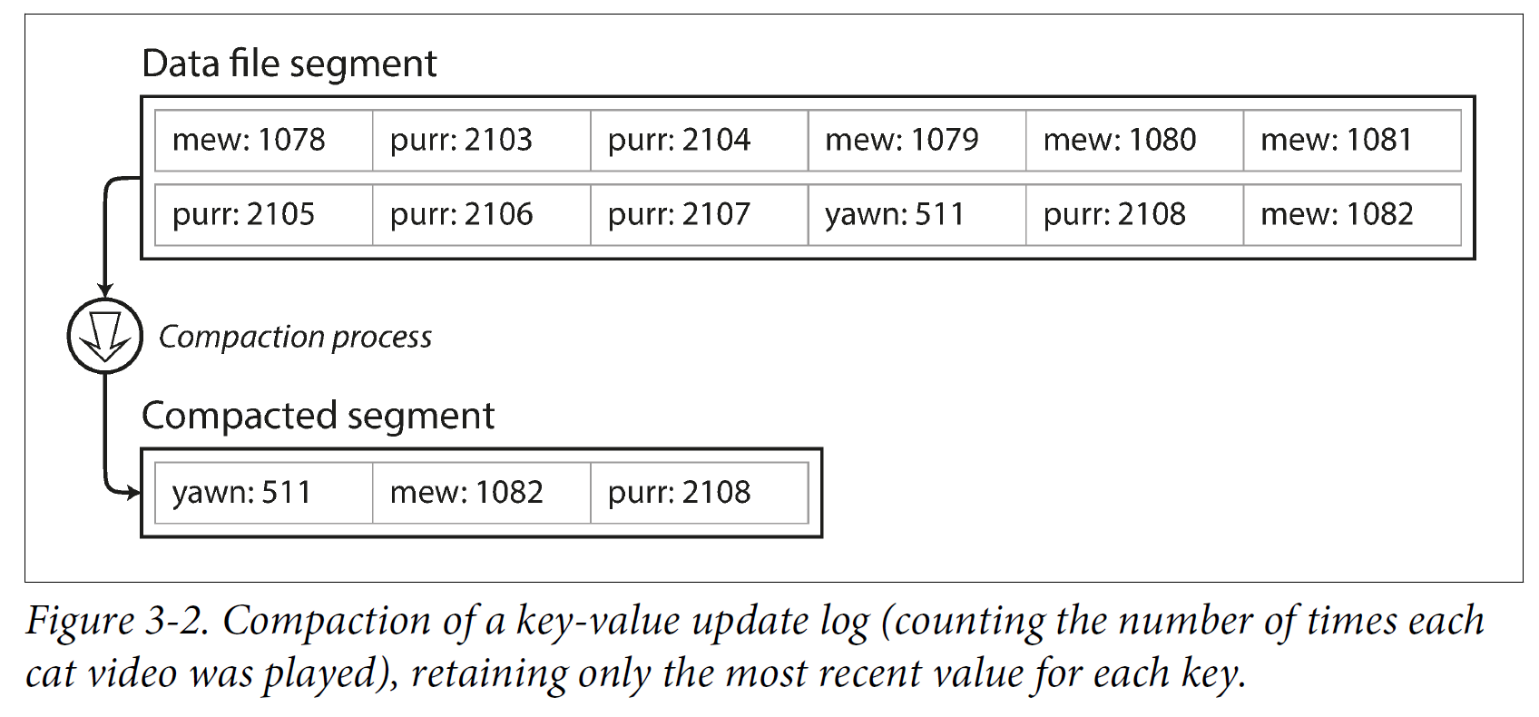
We can then perform compaction on these segments. Compaction means throwing away duplicate keys in the log, and keeping only the most recent update for each key.
-
Moreover, since compaction often makes segments much smaller (assuming that a key is overwritten several times on average within one segment), we can also merge several segments together at the same time as performing the compaction.
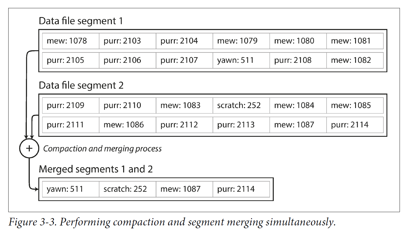
Segments are never modified after they have been written, so the merged segment is written to a new file.
-
The merging and compaction of frozen segments can be done in a background thread, and while it is going on, we can still continue to serve read and write requests as normal, using the old segment files.
-
After the merging process is complete, we switch read requests to using the new merged segment instead of the old segments—and then the old segment files can simply be deleted.
-
Each segment now has its own in-memory hash table, mapping keys to file offsets. In order to find the value for a key, we first check the most recent segment’s hash map; if the key is not present we check the second-most-recent segment, and so on. The merging process keeps the number of segments small, so lookups don’t need to check many hash maps.
2. SSTables and LSM-Trees
In each log-structured storage segment is a sequence of key-value pairs. These pairs appear in the order that they were written, and values later in the log take precedence over values for the same key earlier in the log. Apart from that, the order of key-value pairs in the file does not matter.
Now we can make a simple change to the format of our segment files: we require that the sequence of key-value pairs is sorted by key. At first glance, that requirement seems to break our ability to use sequential writes, but we’ll get to that in a moment.
We call this format Sorted String Table, or SSTable for short. We also require that each key only appears once within each merged segment file (the compaction process already ensures that). SSTables have several big advantages over log segments with hash indexes:
-
Merging segments is simple and efficient, even if the files are bigger than the available memory.
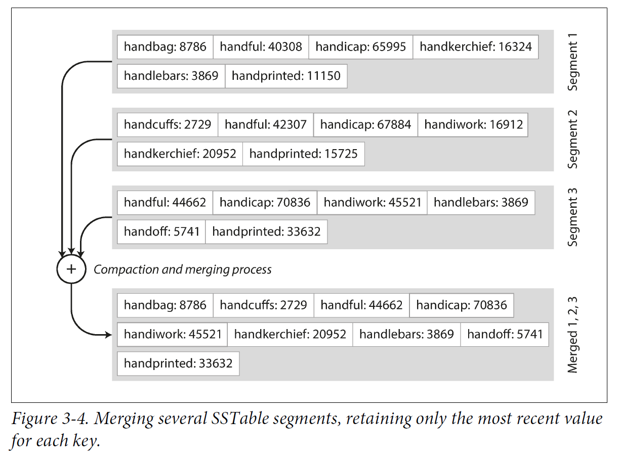
The approach is like the one used in the merge-sort algorithm: you start reading the input files side by side, look at the first key in each file, copy the lowest key (according to the sort order) to the output file, and repeat. This produces a new merged segment file, also sorted by key.
When multiple segments contain the same key, we can keep the value from the most recent segment and discard the values in older segments.
-
In order to find a particular key in the file, you no longer need to keep an index of all the keys in memory.
You still need an in-memory index to tell you the offsets for some of the keys, but it can be sparse: one key for every few kilobytes of segment file is sufficient, because a few kilobytes can be scanned very quickly.
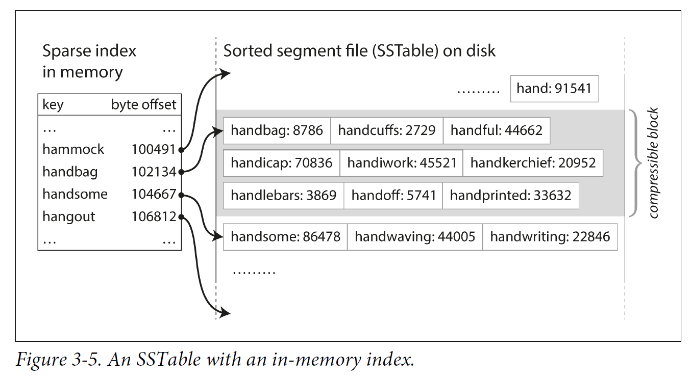
-
Since read requests need to scan over several key-value pairs in the requested range anyway,
-
it is possible to group those records into a block and compress it before writing it to disk.
-
Each entry of the sparse in-memory index then points at the start of a compressed block.
-
Besides saving disk space, compression also reduces the I/O bandwidth use.
-
2.1. Constructing and maintaining SSTables
Maintaining a sorted structure on disk is possible (e.g. “B-Trees”), but maintaining it in memory is much easier. There are plenty of well-known tree data structures that you can use, such as red-black trees or AVL trees. With these data structures, you can insert keys in any order and read them back in sorted order.
We can now make our storage engine work as follows:
-
When a write comes in, add it to an in-memory balanced tree data structure (for example, a red-black tree). This in-memory tree is sometimes called a memtable.
-
When the memtable gets bigger than some threshold—typically a few megabytes —write it out to disk as an SSTable file. This can be done efficiently because the tree already maintains the key-value pairs sorted by key. The new SSTable file becomes the most recent segment of the database. While the SSTable is being written out to disk, writes can continue to a new memtable instance.
-
In order to serve a read request, first try to find the key in the memtable, then in the most recent on-disk segment, then in the next-older segment, etc.
-
From time to time, run a merging and compaction process in the background to combine segment files and to discard overwritten or deleted values.
2.2. Making an LSM-tree out of SSTables
The algorithm described here is essentially what is used in LevelDB and RocksDB, key-value storage engine libraries that are designed to be embedded into other applications. Among other things, LevelDB can be used in Riak as an alternative to Bitcask. Similar storage engines are used in Cassandra and HBase, both of which were inspired by Google’s Bigtable paper (which introduced the terms SSTable and memtable).
Originally this indexing structure was described by Patrick O’Neil et al. under the name Log-Structured Merge-Tree (or LSM-Tree), building on earlier work on log-structured filesystems. Storage engines that are based on this principle of merging and compacting sorted files are often called LSM storage engines.
2.3. Performance optimizations
As always, a lot of detail goes into making a storage engine perform well in practice. For example, the LSM-tree algorithm can be slow when looking up keys that do not exist in the database: you have to check the memtable, then the segments all the way back to the oldest (possibly having to read from disk for each one) before you can be sure that the key does not exist. In order to optimize this kind of access, storage engines often use additional Bloom filters. (A Bloom filter is a memory-efficient data structure for approximating the contents of a set. It can tell you if a key does not appear in the database, and thus saves many unnecessary disk reads for nonexistent keys.)
There are also different strategies to determine the order and timing of how SSTables are compacted and merged. The most common options are size-tiered and leveled compaction. LevelDB and RocksDB use leveled compaction (hence the name of LevelDB), HBase uses size-tiered, and Cassandra supports both. In size-tiered compaction, newer and smaller SSTables are successively merged into older and larger SSTables. In leveled compaction, the key range is split up into smaller SSTables and older data is moved into separate “levels,” which allows the compaction to proceed more incrementally and use less disk space.
Even though there are many subtleties, the basic idea of LSM-trees—keeping a cascade of SSTables that are merged in the background—is simple and effective. Even when the dataset is much bigger than the available memory it continues to work well. Since data is stored in sorted order, you can efficiently perform range queries (scanning all keys above some minimum and up to some maximum), and because the disk writes are sequential the LSM-tree can support remarkably high write throughput.
3. B-Trees
The log-structured indexes we have discussed so far are gaining acceptance, but they are not the most common type of index. The most widely used indexing structure is quite different: the B-tree.
Like SSTables, B-trees keep key-value pairs sorted by key, which allows efficient key-value lookups and range queries. But that’s where the similarity ends: B-trees have a very different design philosophy.
The log-structured indexes we saw earlier break the database down into variable-size segments, typically several megabytes or more in size, and always write a segment sequentially.
By contrast, B-trees break the database down into fixed-size blocks or pages, traditionally 4 KB in size (sometimes bigger), and read or write one page at a time.
-
This design corresponds more closely to the underlying hardware, as disks are also arranged in fixed-size blocks.
-
Each page can be identified using an address or location, which allows one page to refer to another—similar to a pointer, but on disk instead of in memory.
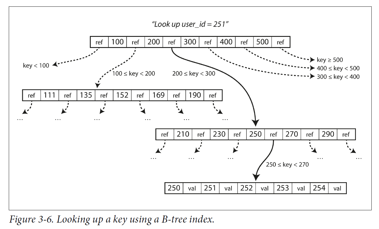
One page is designated as the root of the B-tree; whenever you want to look up a key in the index, you start here.
-
The page contains several keys and references to child pages.
-
Each child is responsible for a continuous range of keys, and the keys between the references indicate where the boundaries between those ranges lie.
-
Eventually we get down to a page containing individual keys (a leaf page), which either contains the value for each key inline or contains references to the pages where the values can be found.
-
The number of references to child pages in one page of the B-tree is called the branching factor.
In practice, the branching factor depends on the amount of space required to store the page references and the range boundaries, but typically it is several hundred.
If you want to update the value for an existing key in a B-tree, you search for the leaf page containing that key, change the value in that page, and write the page back to disk (any references to that page remain valid).
If you want to add a new key, you need to find the page whose range encompasses the new key and add it to that page.
-
If there isn’t enough free space in the page to accommodate the new key, it is split into two half-full pages, and the parent page is updated to account for the new subdivision of key ranges.
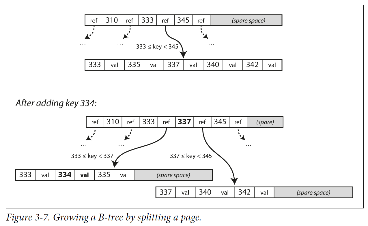
This algorithm ensures that the tree remains balanced: a B-tree with n keys always has a depth of O(log n). Most databases can fit into a B-tree that is three or four levels deep, so you don’t need to follow many page references to find the page you are looking for. (A four-level tree of 4 KB pages with a branching factor of 500 can store up to 256 TB.)
3.1. Making B-trees reliable
The basic underlying write operation of a B-tree is to overwrite a page on disk with new data. It is assumed that the overwrite does not change the location of the page; i.e., all references to that page remain intact when the page is overwritten. This is in stark contrast to log-structured indexes such as LSM-trees, which only append to files (and eventually delete obsolete files) but never modify files in place.
In order to make the database resilient to crashes, it is common for B-tree implementations to include an additional data structure on disk: a write-ahead log (WAL, also known as a redo log). This is an append-only file to which every B-tree modification must be written before it can be applied to the pages of the tree itself. When the database comes back up after a crash, this log is used to restore the B-tree back to a consistent state.
An additional complication of updating pages in place is that careful concurrency control is required if multiple threads are going to access the B-tree at the same time —otherwise a thread may see the tree in an inconsistent state. This is typically done by protecting the tree’s data structures with latches (lightweight locks). Log- structured approaches are simpler in this regard, because they do all the merging in the background without interfering with incoming queries and atomically swap old segments for new segments from time to time.
3.2. B-tree optimizations
-
Instead of overwriting pages and maintaining a WAL for crash recovery, some databases (like LMDB) use a copy-on-write scheme. A modified page is written to a different location, and a new version of the parent pages in the tree is created, pointing at the new location. This approach is also useful for concurency control,
-
We can save space in pages by not storing the entire key, but abbreviating it. Especially in pages on the interior of the tree, keys only need to provide enough information to act as boundaries between key ranges. Packing more keys into a page allows the tree to have a higher branching factor, and thus fewer levels.
-
In general, pages can be positioned anywhere on disk; there is nothing requiring pages with nearby key ranges to be nearby on disk. If a query needs to scan over a large part of the key range in sorted order, that page-by-page layout can be inefficient, because a disk seek may be required for every page that is read. Many B- tree implementations therefore try to lay out the tree so that leaf pages appear in sequential order on disk. However, it’s difficult to maintain that order as the tree grows. By contrast, since LSM-trees rewrite large segments of the storage in one go during merging, it’s easier for them to keep sequential keys close to each other on disk.
-
Additional pointers have been added to the tree. For example, each leaf page may have references to its sibling pages to the left and right, which allows scanning keys in order without jumping back to parent pages.
-
B-tree variants such as fractal trees borrow some log-structured ideas to reduce disk seeks (and they have nothing to do with fractals).
4. References
-
Martin Kleppmann: Designing Data-Intensive Applications, O’Reilly, 2017.