
- 1. Language AI
- 2. Tokens and Embeddings
- 3. Large Language Models
- 4. Text Classification
- 5. Text Clustering and Topic Modeling
- 6. Prompt Engineering
- 7. Advanced Text Generation Techniques and Tools
- 8. Semantic Search and Retrieval-Augmented Generation
- 9. Multimodal Large Language Models
- 10. Creating and Fine-Tuning Text Embedding Models
- References
1. Language AI
|
Google Colab offers free, cloud-based GPU and TPU access for accelerated computation, subject to usage limits, and requires changing the runtime type to GPU to enable it. |
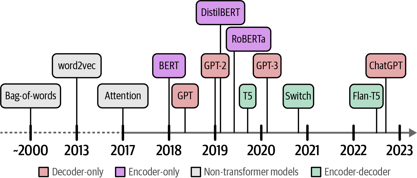
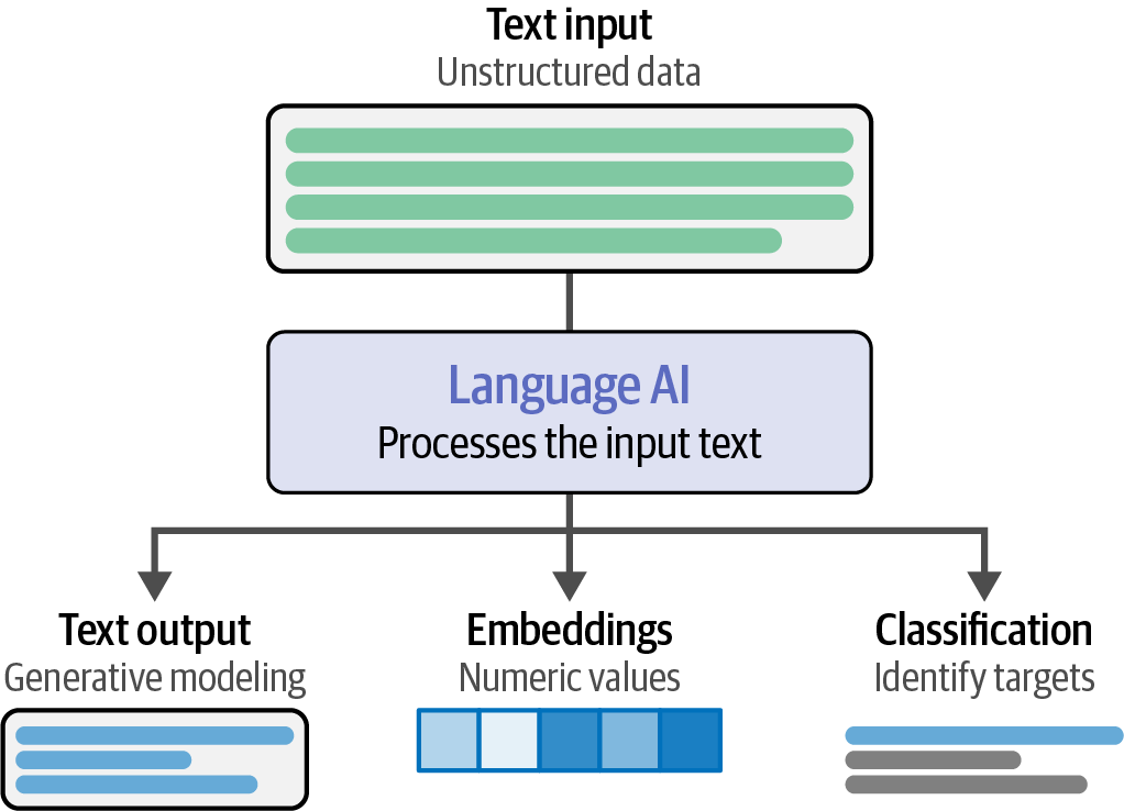
Artificial Intelligence (AI) is the science and engineering of creating intelligent machines, particularly intelligent computer programs, that can perform tasks similar to human intelligence.
Language AI is a subfield of AI focused on developing technologies that can understand, process, and generate human language, which is often used interchangeably with Natural Language Processing (NLP).
-
The Bag-of-Words, a representation model, converts text to numerical vectors by tokenizing it—splitting sentences into individual words or subwords (tokens)—creating a vocabulary, and counting token occurrences to form a vector representation (the 'bag of words').
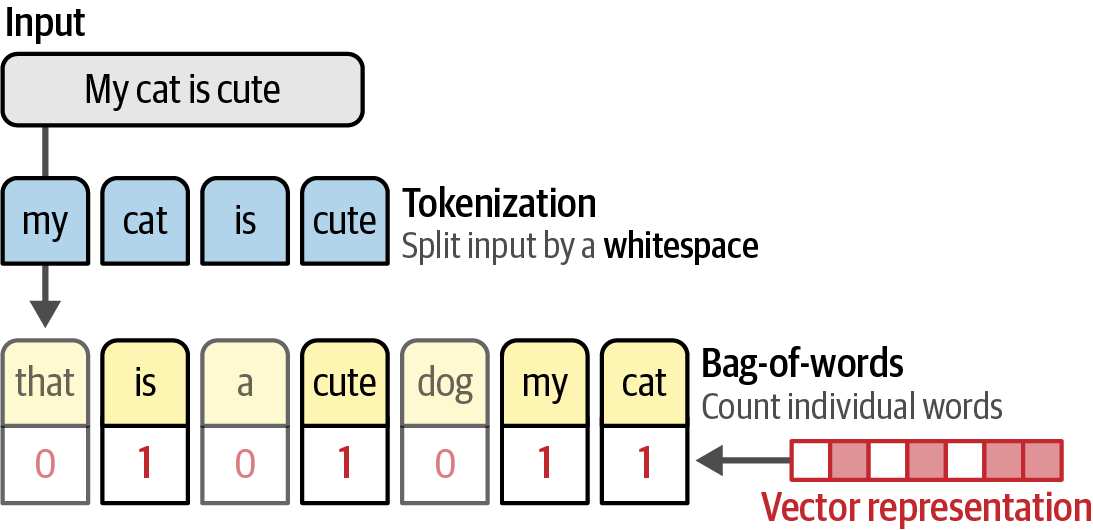 Figure 3. A bag-of-words is created by counting individual words. These values are referred to as vector representations.
 -
Word2vec introduced dense vector embeddings, a significant improvement over Bag-of-Words, by using neural networks to capture the semantic meaning of words based on their context within large datasets, allowing for the measurement of semantic similarity.
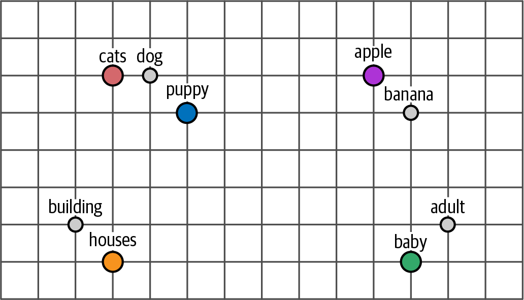 Figure 4. Embeddings of words that are similar will be close to each other in dimensional space.
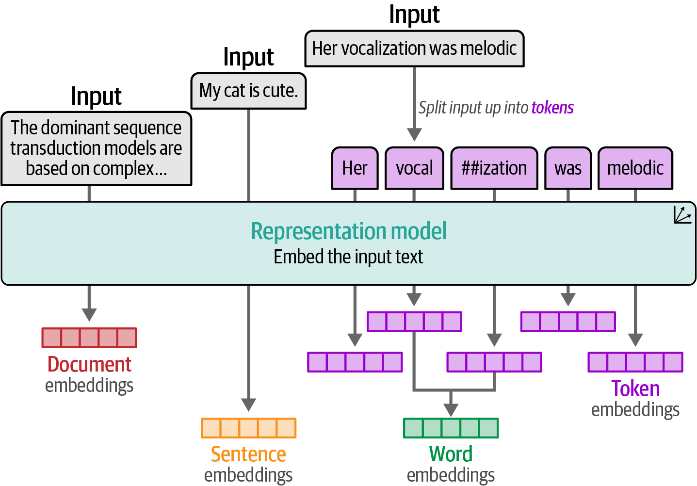 Figure 5. Embeddings can be created for different types of input.
 -
Attention-based Transformer models, replacing RNNs which struggled with long sentences, enabled parallel processing and context-aware language representation by using stacked encoders and decoders to focus on relevant input, revolutionizing language AI.
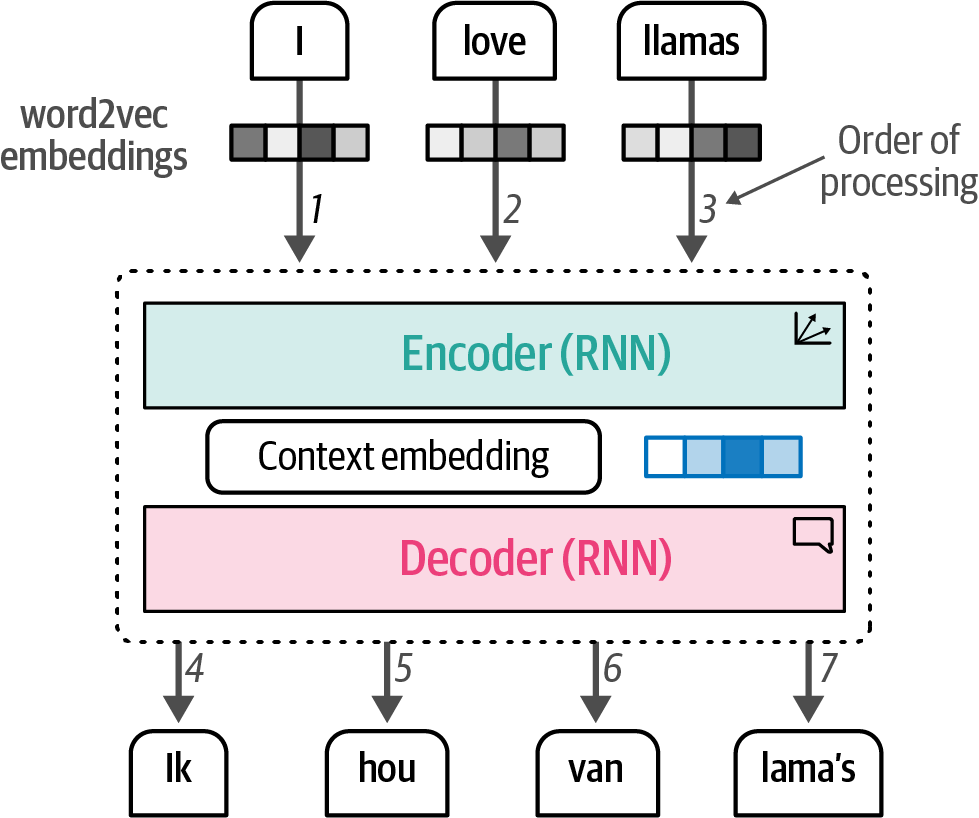 Figure 6. Using word2vec embeddings, a context embedding is generated that represents the entire sequence.
 -
The Transformer is a combination of stacked encoder and decoder blocks where the input flows through each encoder and decoder.
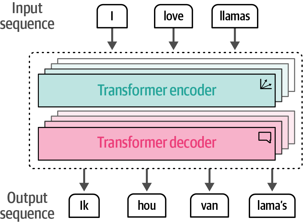 Figure 7. The Transformer is a combination of stacked encoder and decoder blocks where the input flows through each encoder and decoder.
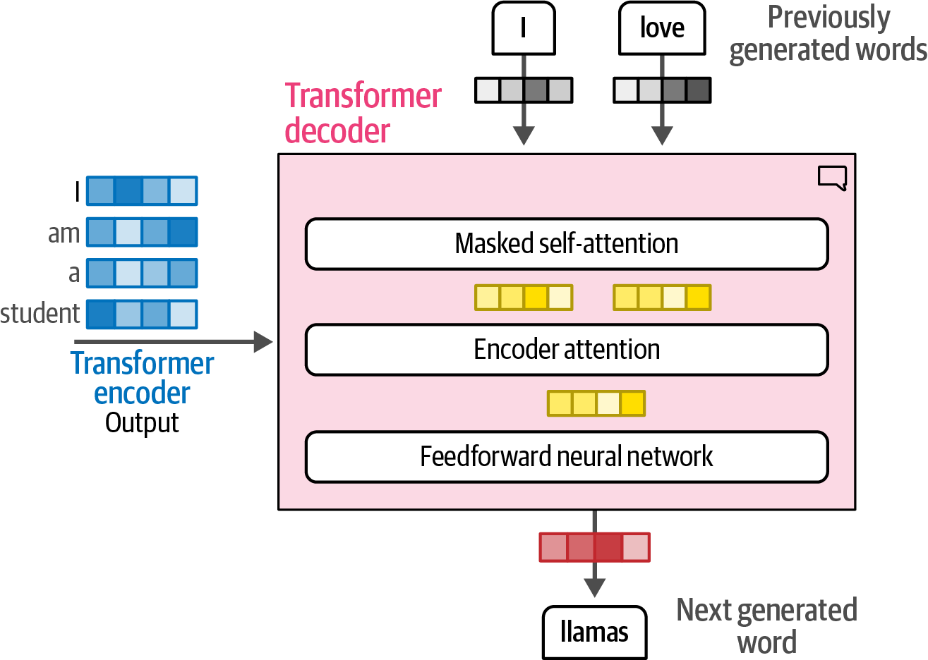 Figure 8. The encoder block revolves around self-attention to generate intermediate representations.
Figure 9. The decoder has an additional attention layer that attends to the output of the encoder.
Figure 8. The encoder block revolves around self-attention to generate intermediate representations.
Figure 9. The decoder has an additional attention layer that attends to the output of the encoder. -
Encoder-only models (a.k.a., representation models) like Bidirectional Encoder Representations from Transformers(BERT) excel at language representation through masked language modeling, while decoder-only models (a.k.a., generative models) like Generative Pre-trained Transformer (GPT) focus on text generation and are the foundation for large language models.
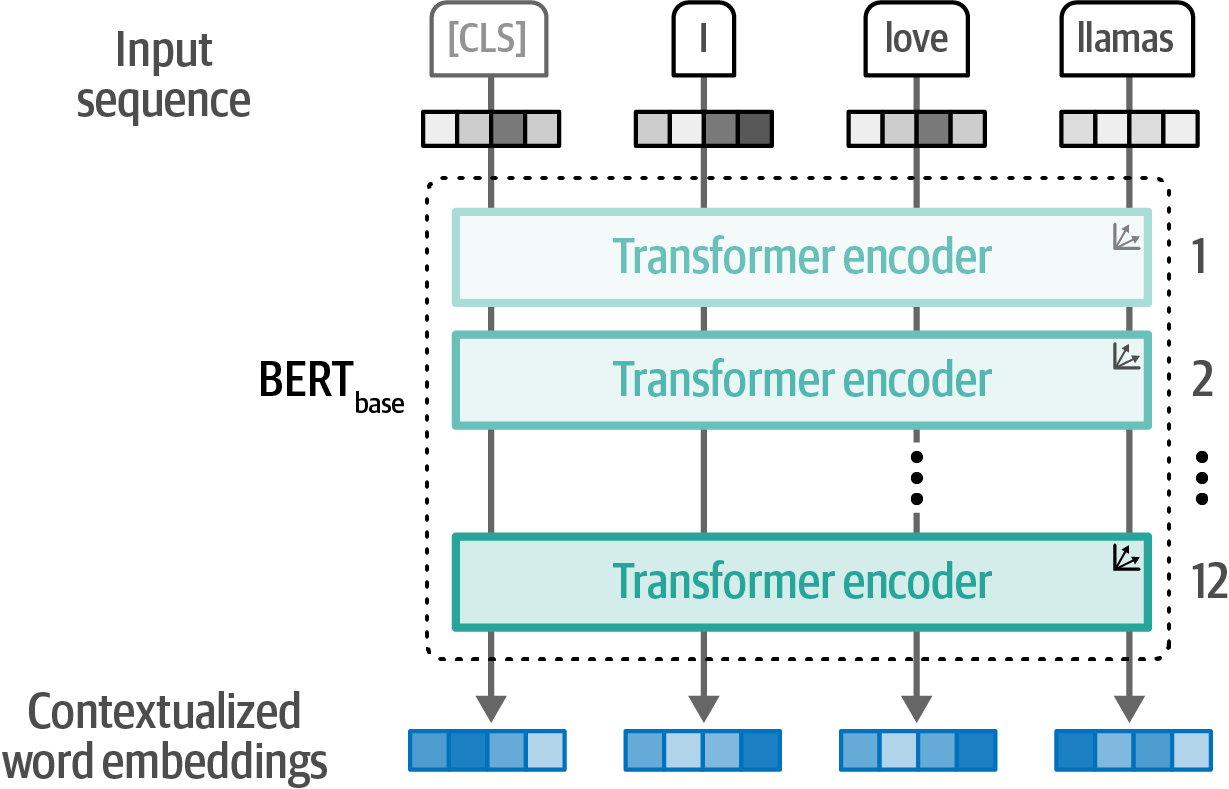 Figure 10. The architecture of a BERT base model with 12 encoders.
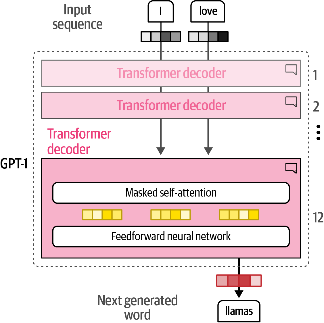 Figure 11. The architecture of a GPT-1. It uses a decoder-only architecture and removes the encoder-attention block.
 -
Generative LLMs function as sequence-to-sequence machines, initially designed for text completion, but their capability to be fine-tuned into chatbots or instruct models that can follow user prompts revealed their true potential.
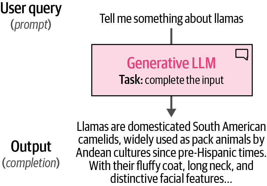 Figure 12. Generative LLMs take in some input and try to complete it. With instruct models, this is more than just autocomplete and attempts to answer the question.
 -
The context length, or window, represents the maximum number of tokens the model can process, enabling the generative LLM to handle larger documents, and the current length expands as the model generates new tokens due to its autoregressive nature.
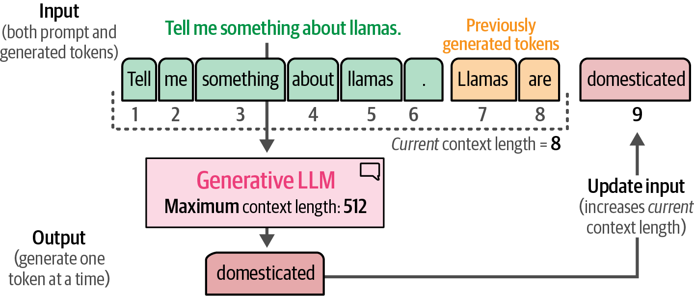 Figure 13. The context length is the maximum context an LLM can handle.
 -
LLMs differ from traditional machine learning by using a two-step training process: pretraining, for general language learning, and fine-tuning (or post-training), to adapt the pretrained (foundation/base) model for specific tasks.
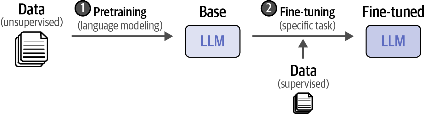 Figure 14. Compared to traditional machine learning, LLM training takes a multistep approach.
 -
Closed-source LLMs, like GPT-4 and Claude, are models that do not have their weights and architecture shared with the public, which are accessed via APIs, and offer high performance with managed hosting, but are costly and limit user control; open LLMs, such as Llama, share their architecture, enabling local use, fine-tuning, and privacy, but require powerful hardware and expertise.
-
The main source for finding and downloading LLMs is the Hugging Face Hub. Hugging Face is the organization behind the well-known Transformers package, which for years has driven the development of language models in general.
# If a connection to the Hugging Face URL (https://huggingface.co/) fails, try to set the HF_ENDPOINT environment variable to the mirror URL. import os os.environ["HF_ENDPOINT"] = "https://hf-mirror.com" -
Hugging Face, the organization behind the Transformers package, is the primary source for finding and downloading LLMs, built upon the Transformer framework.
import os
from transformers import AutoModelForCausalLM, AutoTokenizer, pipeline

# HF_ENDPOINT controls the base URL used by the transformers library
# to download models and other resources from the Hugging Face Hub.
os.environ['HF_ENDPOINT'] = 'https://hf-mirror.com'

# determine the device
dev = 'cuda' if torch.cuda.is_available() else 'cpu'

# load model and tokenizer
MODEL_NAME = 'microsoft/Phi-4-mini-instruct'
model = AutoModelForCausalLM.from_pretrained(
    MODEL_NAME,
    torch_dtype='auto',
    device_map=dev,
    trust_remote_code=True,
)
tokenizer = AutoTokenizer.from_pretrained(MODEL_NAME)

# create a pipeline
pipe = pipeline(
    "text-generation",
    model=model,
    tokenizer=tokenizer,
    return_full_text=False,
    max_new_tokens=500,
    do_sample=True,
)

# the prompt (user input / query)
messages = [{"role": "user", "content": "Create a funny joke about chickens."}]

# generate output
output = pipe(messages)
print(output[0]["generated_text"])
Why did the chicken join the band? Because he heard they had the "cluck-loudest" performers around!# clear memory and empty the VRAM import gc import torch # attempt to delete the model, tokenizer, and pipeline objects from memory del model, tokenizer, pipe # flush memory gc.collect() if torch.cuda.is_available(): # if a GPU is available, empty the CUDA cache to free up GPU memory torch.cuda.empty_cache()
2. Tokens and Embeddings
Tokens and embeddings are two of the central concepts of using large language models (LLMs).
2.1. LLM Tokenization
import os
import torch
from transformers import AutoModelForCausalLM, AutoTokenizer, pipeline

# HF_ENDPOINT controls the base URL used by the transformers library
# to download models and other resources from the Hugging Face Hub.
os.environ['HF_ENDPOINT'] = 'https://hf-mirror.com'

# determine the device
dev = 'cuda' if torch.cuda.is_available() else 'cpu'

# load model and tokenizer
MODEL_NAME = 'microsoft/Phi-4-mini-instruct'
model = AutoModelForCausalLM.from_pretrained(
    MODEL_NAME,
    torch_dtype='auto',
    device_map=dev,
    trust_remote_code=True,
)
tokenizer = AutoTokenizer.from_pretrained(MODEL_NAME)

prompt = '<s> Write an email apologizing to Sarah for the tragic gardening mishap. Explain how it happened.<|assistant|>'

# tokenize the input prompt
input_ids = tokenizer(prompt, return_tensors='pt').input_ids.to(dev)
print(f'input_ids: {input_ids}')

# generate the text
output_ids = model.generate(input_ids=input_ids, max_new_tokens=20)
print(f'output_ids: {output_ids}')

# print the output
print(tokenizer.decode(output_ids[0]))
input_ids: tensor([[101950, 29, 16465, 448, 3719, 39950, 6396, 316, 32145,
395, 290, 62374, 66241, 80785, 403, 13, 115474, 1495,
480, 12570, 13, 200019]])
output_ids: tensor([[101950, 29, 16465, 448, 3719, 39950, 6396, 316, 32145,
395, 290, 62374, 66241, 80785, 403, 13, 115474, 1495,
480, 12570, 13, 200019, 18174, 25, 336, 2768, 512,
6537, 10384, 395, 290, 193145, 147276, 403, 279, 36210,
32145, 4464, 40, 5498, 495, 3719]])
<s> Write an email apologizing to Sarah for the tragic gardening mishap. Explain how it happened.<|assistant|>Subject: Sincere Apologies for the Gardening Mishap
Dear Sarah,
I hope this email-
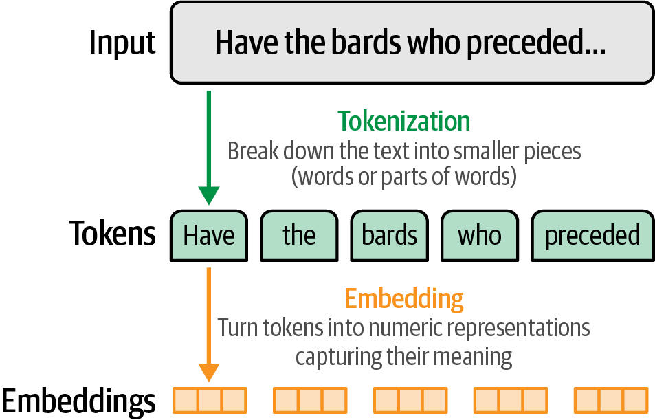
Tokens, the units into which text prompts are broken for model input, also form the model’s output.
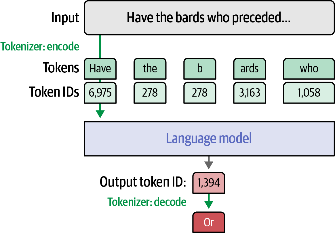 Figure 16. A tokenizer encodes input prompts into token ID lists for the language model and decodes the model’s output token IDs back into words or tokens.
-
Each ID corresponds to a specific token (character, word, or subword) in the tokenizer’s vocabulary.
-
The tokenizer’s vocabulary acts as a lookup table, allowing the model to convert between text and these integer representations.
for id in [101950, 29, 16465, 448, 3719, 39950]:
    print(tokenizer.decode(id))
# <s
# >
#  Write
#  an
#  email
#  apolog

for id in [18174, 25, 336, 2768, 512]:
    print(tokenizer.decode(id)
# Subject
# :
#  S
# inc
# ere
-
-
Tokenization is determined by three major design decisions: the tokenizer algorithm (e.g., BPE, WordPiece, SentencePiece), tokenization parameters (including vocabulary size, special tokens, capitalization, treatment of capitalization and different languages), and the dataset the tokenizer is trained on (a tokenizer trained on an English text dataset will be different from another trained on a code dataset or a multilingual text dataset).
-
Tokenization methods vary in granularity, from word-level to byte-level, with subword tokenization offering a balance of vocabulary expressiveness and efficiency, making it the most common approach in modern language models.
2.2. Token Embeddings
Text --> Tokens --> Token IDs --> Embeddings (Vectors)-
A tokenizer, once trained, becomes intrinsically linked to its language model during the model’s training; consequently, a pretrained language model cannot function with a different tokenizer without retraining, as their vocabularies and tokenization schemes are aligned.
-
An embedding is a dense, numerical vector representation of a token (like a word or subword) that captures its semantic meaning within a high-dimensional space, enabling language models to understand and process relationships between words.
-
A language model stores static embedding vectors for each token in its vocabulary, but also generates contextualized word embeddings, dynamically representing a token based on its context instead of a single, fixed vector.
-
A language model holds an embedding vector associated with each token in its tokenizer.
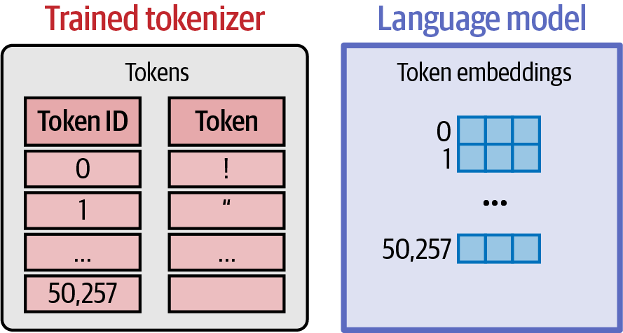 Figure 17. A language model holds an embedding vector associated with each token in its tokenizer.
 -
A language model operates on raw, static embeddings as its input and produces contextual text embeddings.
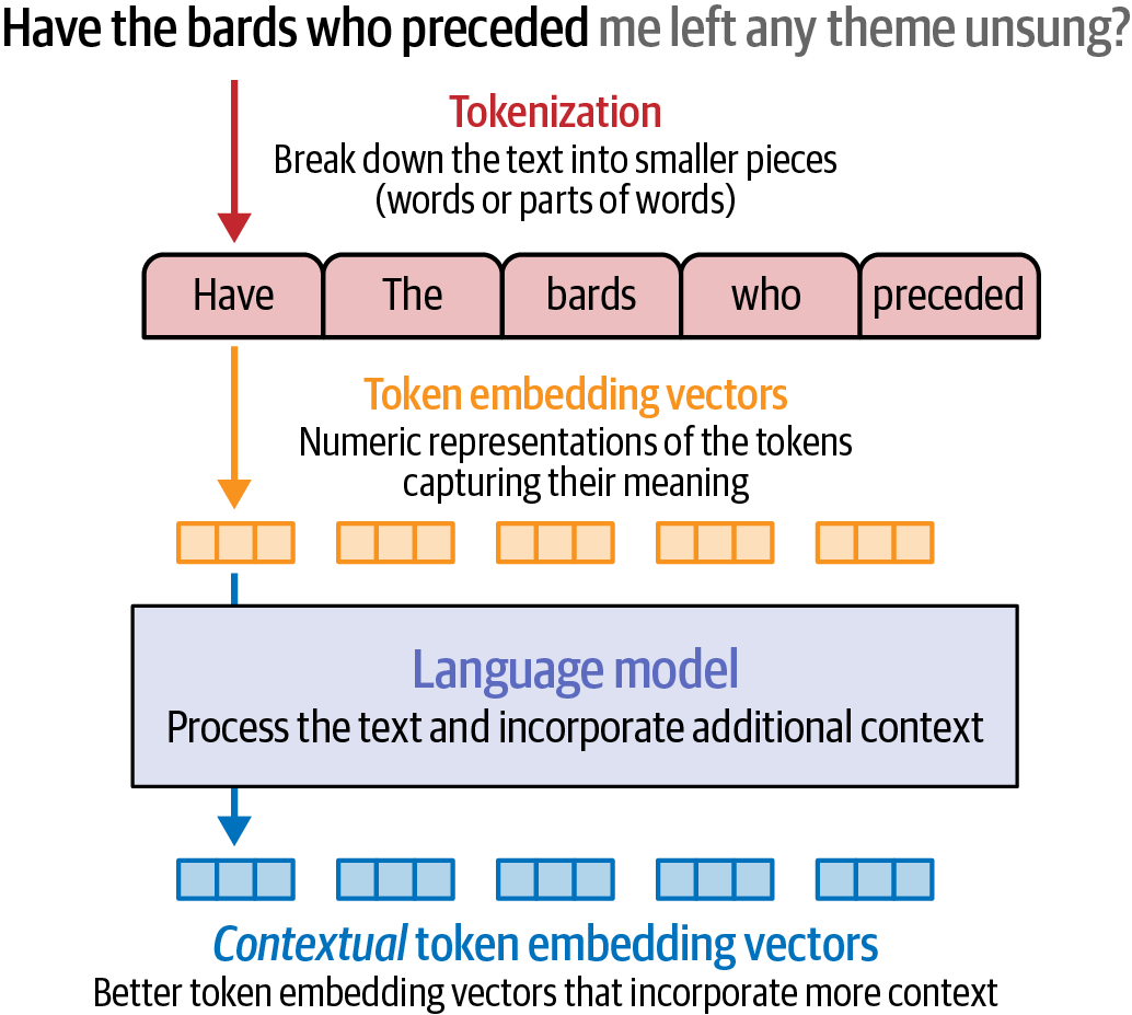 Figure 18. A language model operates on raw, static embeddings as its input and produces contextual text embeddings.
from transformers import AutoModel, AutoTokenizer

# load a tokenizer
tokenizer = AutoTokenizer.from_pretrained('microsoft/deberta-base')

# load a language model
model = AutoModel.from_pretrained('microsoft/deberta-v3-xsmall')

# tokenize the sentence: convert text to token IDs
tokens = tokenizer('Hello world', return_tensors='pt')

# print the decoded tokens to show tokenization
for token_id in tokens['input_ids'][0]:
    print(tokenizer.decode(token_id))
print('\n')

# process the token IDs through the model to get contextualized embeddings
output = model(**tokens)[0]

# show the shape of the embedding result
print(f'{output.shape}\n')

# output contains the contextualized embedding vectors
print(output)
[CLS] Hello world [SEP] torch.Size([1, 4, 384]) tensor([[[-3.4816, 0.0861, -0.1819, ..., -0.0612, -0.3911, 0.3017], [ 0.1898, 0.3208, -0.2315, ..., 0.3714, 0.2478, 0.8048], [ 0.2071, 0.5036, -0.0485, ..., 1.2175, -0.2292, 0.8582], [-3.4278, 0.0645, -0.1427, ..., 0.0658, -0.4367, 0.3834]]], grad_fn=<NativeLayerNormBackward0>)
-
2.3. Text Embeddings
Text embeddings are single, dense vectors that represent the semantic meaning of entire sentences, paragraphs, or documents, in contrast to token embeddings, which represent individual words or subwords.
from sentence_transformers import SentenceTransformer

# load model
model = SentenceTransformer('sentence-transformers/all-MiniLM-L6-v2')

# convert text to text embeddings
embeddings = model.encode("Best movie ever!")

print(embeddings.shape) # (384,)|
Input Sequence Length: https://www.sbert.net/
For transformer models like BERT, RoBERTa, DistilBERT etc., the runtime and memory requirement grows quadratic with the input length. This limits transformers to inputs of certain lengths. A common value for BERT-based models are 512 tokens, which corresponds to about 300-400 words (for English). Each model has a maximum sequence length under |
3. Large Language Models
import torch
from transformers import AutoModelForCausalLM, AutoTokenizer, pipeline

# determine the device
dev = 'cuda' if torch.cuda.is_available() else 'cpu'

# load model and tokenizer
MODEL_NAME = 'microsoft/Phi-4-mini-instruct'
model = AutoModelForCausalLM.from_pretrained(
    MODEL_NAME,
    torch_dtype='auto',
    device_map=dev,
    trust_remote_code=True,
)
tokenizer = AutoTokenizer.from_pretrained(MODEL_NAME)

# create a pipeline
generator = pipeline(
    "text-generation",
    model=model,
    tokenizer=tokenizer,
    return_full_text=False,
    max_new_tokens=50,
    do_sample=False,
)
3.1. Inputs and Outputs
The most common picture of understanding the behavior of a Transformer LLM is to think of it as a software system that takes in text and generates text in response.
-
Once a large enough text-in-text-out model is trained on a large enough high-quality dataset, it becomes able to generate impressive and useful outputs.
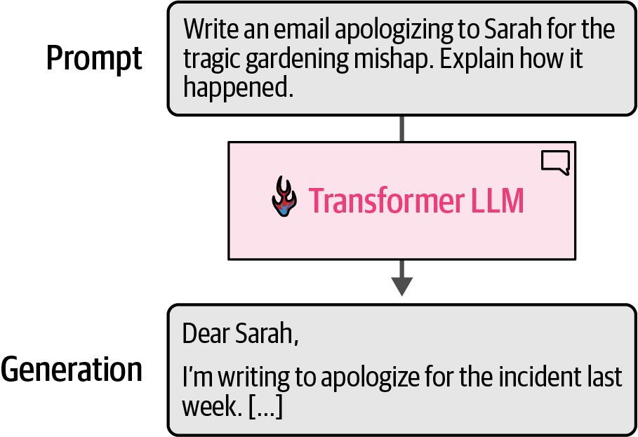 Figure 19. At a high level of abstraction, Transformer LLMs take a text prompt and output generated text.
 -
The model does not generate the text all in one operation; it actually generates one token at a time.
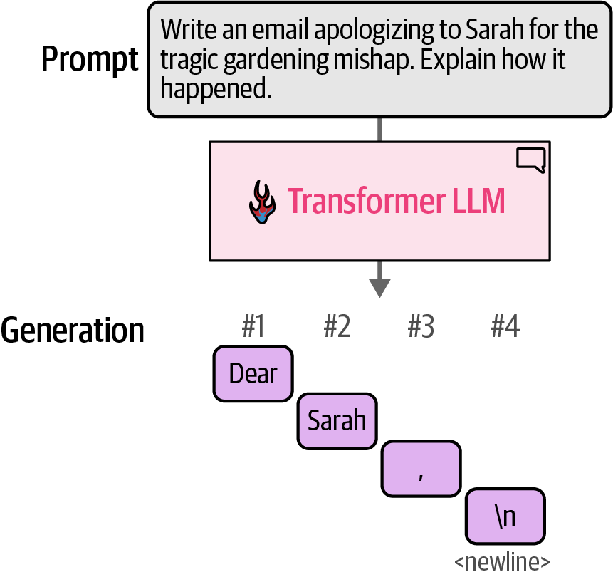 Figure 20. Transformer LLMs generate one token at a time, not the entire text at once.
 -
Each token generation step is one forward pass through the model (that’s machine-learning speak for the inputs going into the neural network and flowing through the computations it needs to produce an output on the other end of the computation graph).
-
After each token generation, the input prompt for the next generation step is tweaked by appending the output token to the end of the input prompt.
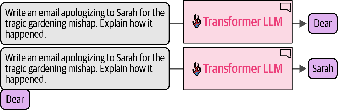 Figure 21. An output token is appended to the prompt, then this new text is presented to the model again for another forward pass to generate the next token.
 -
Text generation LLMs are called autoregressive models because they generate text sequentially, using prior outputs as input, unlike text representation models like BERT, which process the entire input at once.
3.2. Components
-
A language model consists of a tokenizer, a stack of Transformer blocks for processing, and an LM head that converts the processed information into probability scores for the next token.
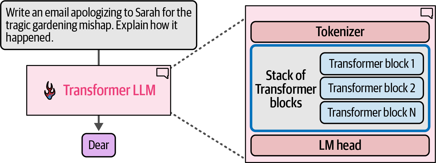 Figure 22. A Transformer LLM is made up of a tokenizer, a stack of Transformer blocks, and a language modeling head.
 -
The model has a vector representation associated with each of these tokens in the vocabulary (token embeddings).
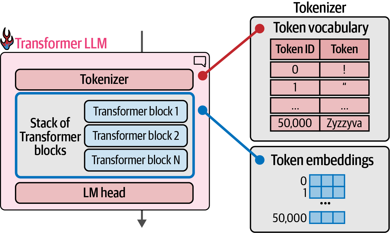 Figure 23. The tokenizer has a vocabulary of 50,000 tokens. The model has token embeddings associated with those embeddings.
 -
For each generated token, the process flows once through each of the Transformer blocks in the stack in order, then to the LM head, which finally outputs the probability distribution for the next token.
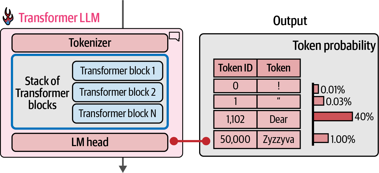 Figure 24. At the end of the forward pass, the model predicts a probability score for each token in the vocabulary.
import torch
from transformers import AutoModelForCausalLM, AutoTokenizer, pipeline

# determine the device
dev = 'cuda' if torch.cuda.is_available() else 'cpu'

# load model and tokenizer
MODEL_NAME = 'microsoft/Phi-4-mini-instruct'
model = AutoModelForCausalLM.from_pretrained(
    MODEL_NAME,
    torch_dtype='auto',
    device_map=dev,
    trust_remote_code=True,
)
print(model)
Phi3ForCausalLM( (model): Phi3Model( (embed_tokens): Embedding(200064, 3072, padding_idx=199999) (layers): ModuleList( (0-31): 32 x Phi3DecoderLayer( (self_attn): Phi3Attention( (o_proj): Linear(in_features=3072, out_features=3072, bias=False) (qkv_proj): Linear(in_features=3072, out_features=5120, bias=False) ) (mlp): Phi3MLP( (gate_up_proj): Linear(in_features=3072, out_features=16384, bias=False) (down_proj): Linear(in_features=8192, out_features=3072, bias=False) (activation_fn): SiLU() ) (input_layernorm): Phi3RMSNorm((3072,), eps=1e-05) (post_attention_layernorm): Phi3RMSNorm((3072,), eps=1e-05) (resid_attn_dropout): Dropout(p=0.0, inplace=False) (resid_mlp_dropout): Dropout(p=0.0, inplace=False) ) ) (norm): Phi3RMSNorm((3072,), eps=1e-05) (rotary_emb): Phi3RotaryEmbedding() ) (lm_head): Linear(in_features=3072, out_features=200064, bias=False) )
3.3. Probability Distribution (Sampling/Decoding)
Language models use a probability distribution to determine the next token, which is called the decoding strategy.
-
The easiest strategy would be to always pick the token with the highest probability score, which is called greedy decoding (equivalent to setting the temperature to zero in an LLM).
In practice, this doesn’t tend to lead to the best outputs for most use cases.
-
A better approach is to introduce randomness by sampling from the probability distribution, sometimes choosing the second or third highest probability token.
3.4. Parallel Token Processing and Context Size
-
Transformers excel at parallel processing, unlike earlier architectures, which is evident in how they handle token generation.
-
Each input token is processed simultaneously through its own computation path or stream.
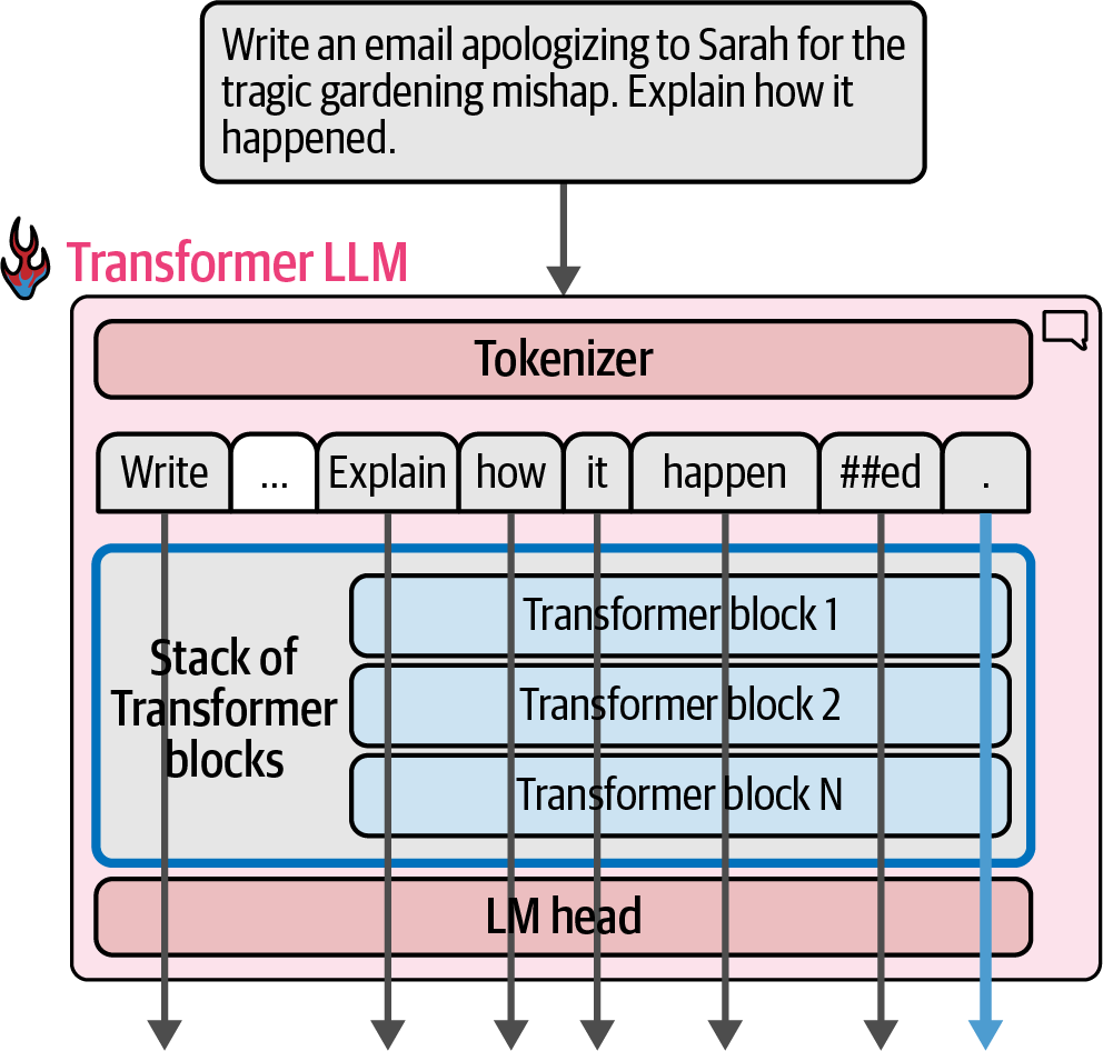 Figure 25. Each token is processed through its own stream of computation (with some interaction between them in attention steps).
 -
A model with 4K context length or context size can only process 4K tokens and would only have 4K of these streams.
-
-
Each of the token streams starts with an input vector (the embedding vector and some positional information).
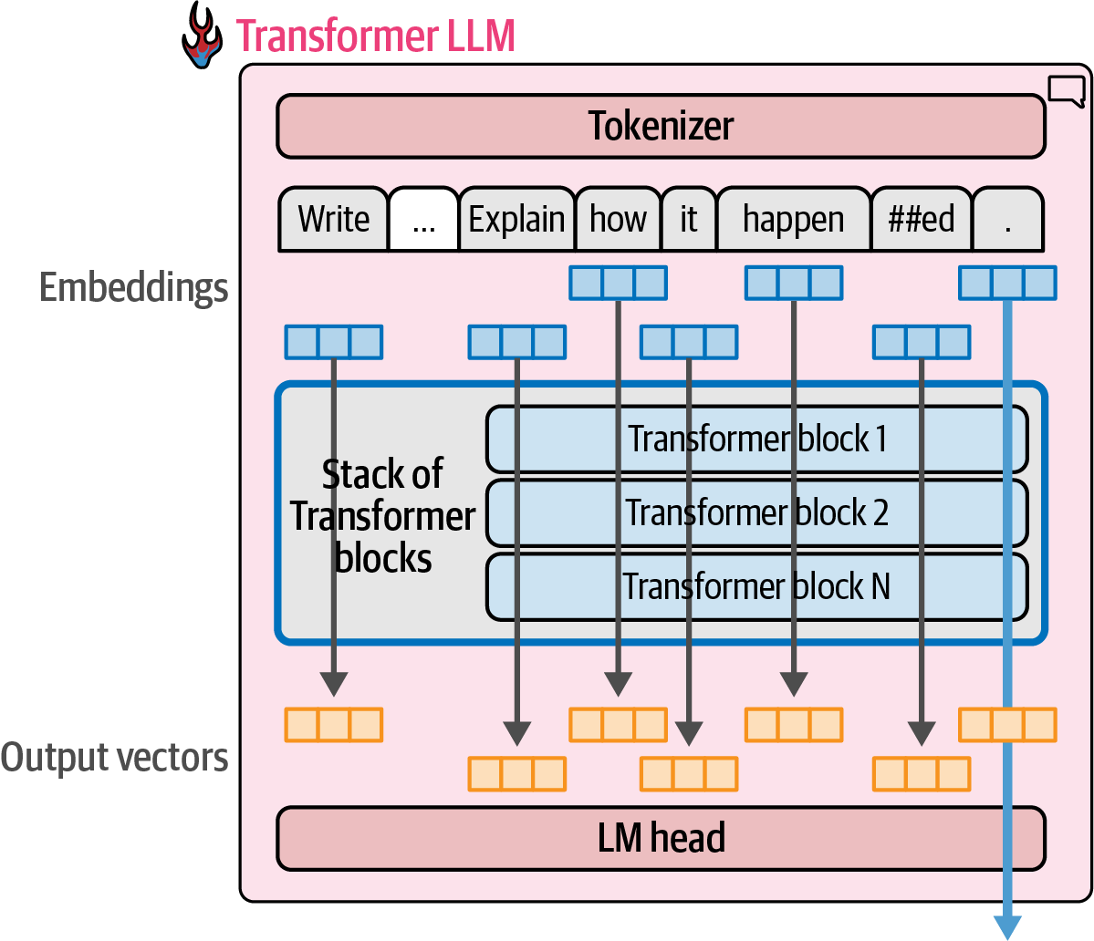 Figure 26. Each processing stream takes a vector as input and produces a final resulting vector of the same size (often referred to as the model dimension).
-
At the end of the stream, another vector emerges as the result of the model’s processing.
-
For text generation, only the output result of the last stream is used to predict the next token.
-
That output vector is the only input into the LM head as it calculates the probabilities of the next token.
-
-
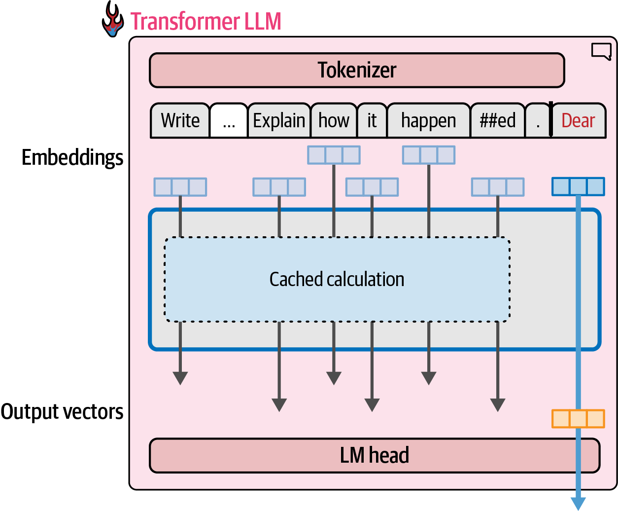
3.5. Keys and Values Caching
Transformer models use a key/value (KV) cache to cache the results of the previous calculation (especially some of the specific vectors in the attention mechanism), speeding up text generation by avoiding redundant calculations.
-
In Hugging Face Transformers, cache is enabled by default, and can be disabled it by setting
use_cachetoFalse.prompt = 'Write a very long email apologizing to Sarah for the tragic gardening mishap. Explain how it happened.' input_ids = tokenizer(prompt, return_tensors='pt').input_ids.to(dev) generation_output = model.generate( input_ids=input_ids, max_new_tokens=100, use_cache=False, )
3.6. Transformer Block
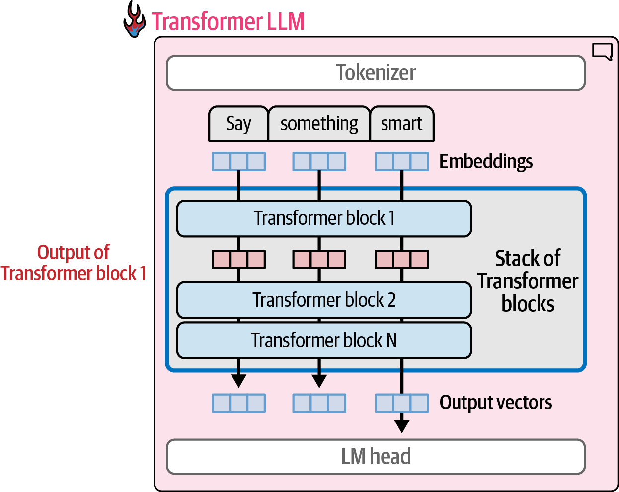
Transformer LLMs are composed of a series Transformer blocks (often in the range of six in the original Transformer paper, to over a hundred in many large LLMs) and each block processes its inputs, then passes the results of its processing to the next block.
-
A Transformer block is made up of two successive components:
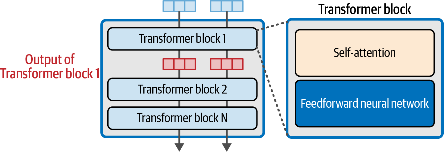 Figure 29. A Transformer block is made up of a self-attention layer and a feedforward neural network.
-
The attention layer is mainly concerned with incorporating relevant information from other input tokens and positions
-
The feedforward layer houses the majority of the model’s processing capacity
-
-
The feedforward network in a Transformer model stores learned information, such as 'The Shawshank' and 'Redemption,' and enables interpolation and generalization for generating text on unseen inputs.
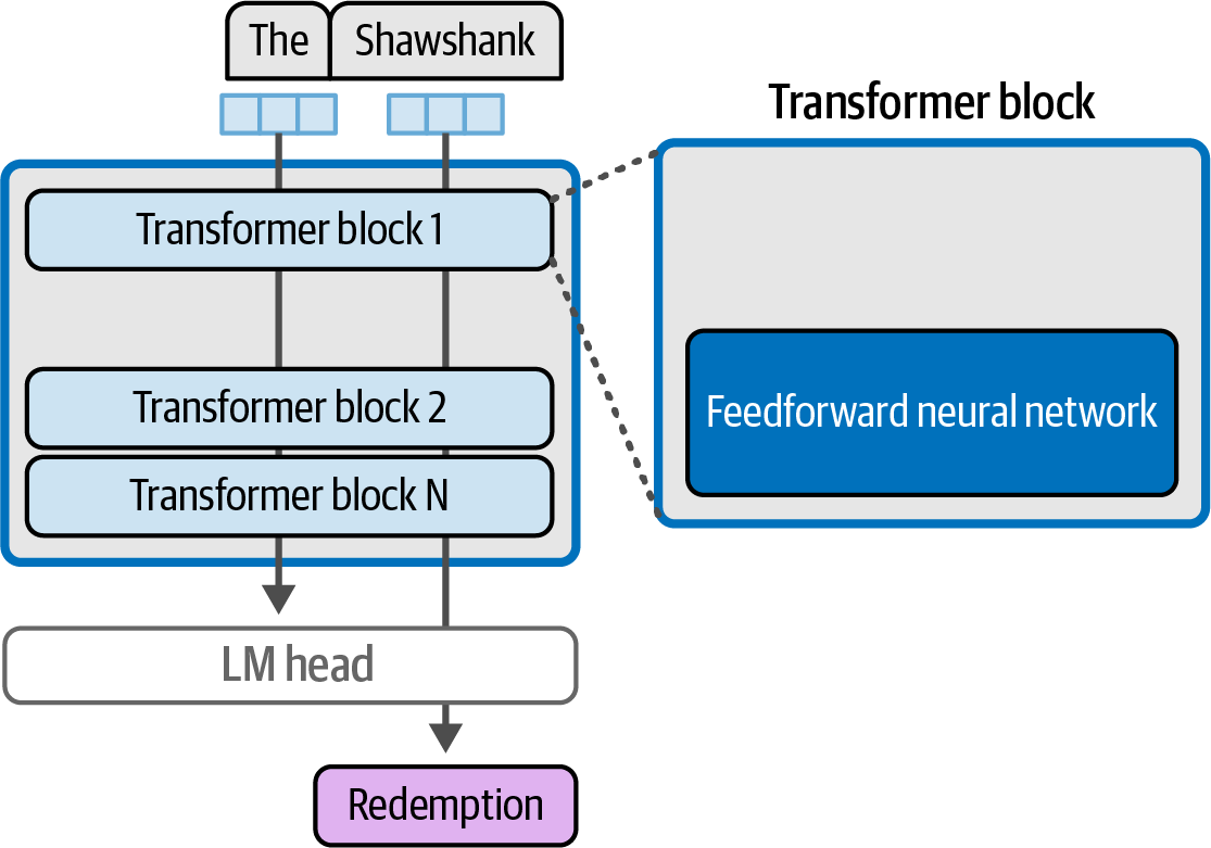 Figure 30. The feedforward neural network component of a Transformer block likely does the majority of the model’s memorization and interpolation.
 -
The attention layer in a Transformer model enables context awareness, crucial for language understanding beyond simple memorization.
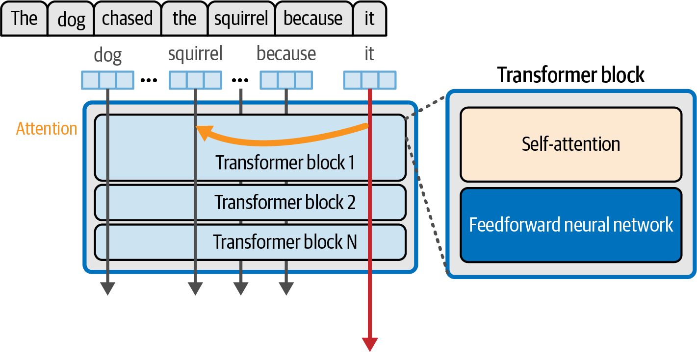 Figure 31. The self-attention layer incorporates relevant information from previous positions that help process the current token.
4. Text Classification
A common task in natural language processing is classification, where the goal is to train a model to assign a label or class to input text, a technique widely used in applications like sentiment analysis and intent detection, significantly impacted by both representative and generative language models.
The Hugging Face Hub is a collaborative platform for machine learning resources (models, datasets, applications), and the datasets package can be used to load datasets.
The dataset is split into train (for training), test (for final evaluation), and validation (for intermediate generalization checks, especially during hyperparameter tuning).
from datasets import load_dataset

# load data
data = load_dataset("rotten_tomatoes") # the well-known 'rotten_tomatoes' dataset
data
DatasetDict({
train: Dataset({
features: ['text', 'label'],
num_rows: 8530
})
validation: Dataset({
features: ['text', 'label'],
num_rows: 1066
})
test: Dataset({
features: ['text', 'label'],
num_rows: 1066
})
})4.1. Representation Models
-
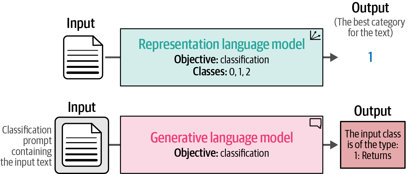
Classification with pretrained representation models generally comes in two flavors, either using a task-specific model or an embedding model.
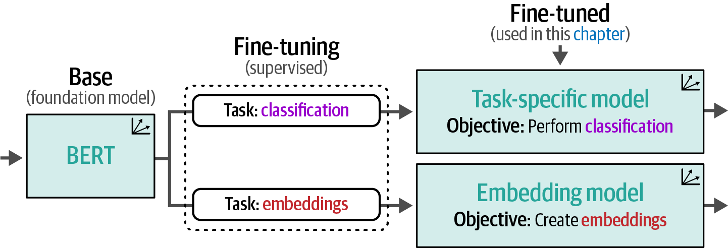 Figure 33. A foundation model is fine-tuned for specific tasks; for instance, to perform classification or generate general-purpose embeddings.
 -
A task-specific model is a representation model, such as BERT, trained for a specific task, like sentiment analysis.
-
An embedding model generates general-purpose embeddings that can be used for a variety of tasks not limited to classification, like semantic search.
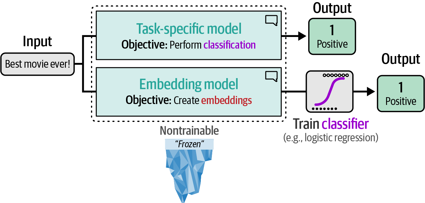 Figure 34. Perform classification directly with a task-specific model or indirectly with general-purpose embeddings.
4.1.1. Task-Specific Model
from datasets import load_dataset

# load the well-known 'rotten_tomatoes' dataset for sentiment analysis
data = load_dataset("rotten_tomatoes")

# determine the device to use for computation (GPU if available, otherwise CPU)
import torch
dev = 'cuda' if torch.cuda.is_available() else 'cpu'

from transformers import pipeline

# specify the path to the pre-trained Twitter-RoBERTa-base for Sentiment Analysis model
model_path = "cardiffnlp/twitter-roberta-base-sentiment-latest"
# load the pre-trained sentiment analysis model into a pipeline for easy inference
pipe = pipeline(
    model=model_path,
    tokenizer=model_path,
    return_all_scores=True, # return the scores for all sentiment labels
    device=dev, # specify the device to run the pipeline on
)

import numpy as np
from tqdm import tqdm # for progress bar during inference
from transformers.pipelines.pt_utils import KeyDataset # utility to feed data to the pipeline

# run inference on the test dataset
y_pred = [] # list to store the predicted sentiment labels
for output in tqdm(
    # iterate through the 'text' column of the test dataset
    pipe(KeyDataset(data["test"], "text")), total=len(data["test"])
):
    # extract the negative sentiment score
    negative_score = output[0]["score"]
    # extract the positive sentiment score (assuming labels are ordered: negative, neutral, positive)
    positive_score = output[2]["score"]
    # predict the sentiment based on the highest score (0 for negative, 1 for positive)
    assignment = np.argmax([negative_score, positive_score])
    # add the predicted label to the list
    y_pred.append(assignment)

from sklearn.metrics import classification_report


def evaluate_performance(y_true, y_pred):
    '''Create and print the classification report comparing true and predicted labels'''
    performance = classification_report(
        y_true, y_pred, target_names=["Negative Review", "Positive Review"]
    )
    print(performance)


# evaluate the performance of the sentiment analysis model on the test set
evaluate_performance(data["test"]["label"], y_pred) # compare the true labels with the predicted labels
precision recall f1-score support
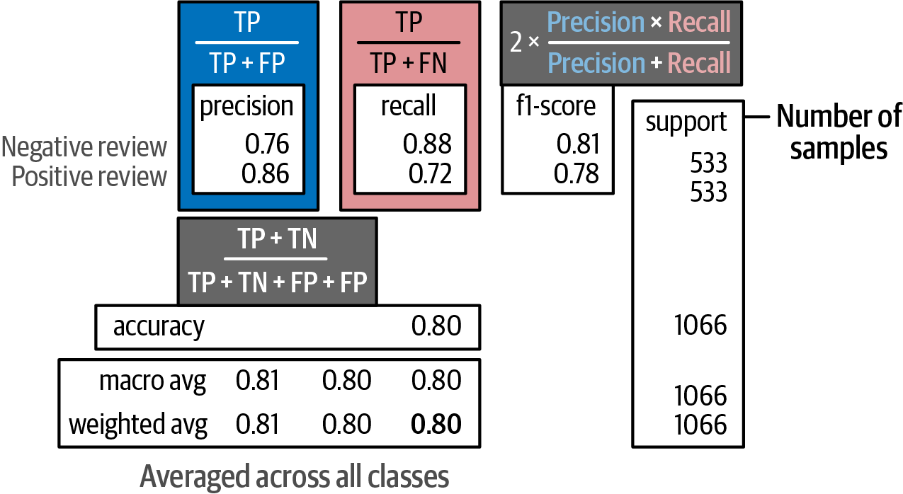
Negative Review 0.76 0.88 0.81 533
Positive Review 0.86 0.72 0.78 533
accuracy 0.80 1066
macro avg 0.81 0.80 0.80 1066
weighted avg 0.81 0.80 0.80 1066The above generated classification report shows four such methods: precision, recall, accuracy, and the F1 score.
-
Precision measures how many of the items found are relevant, which indicates the accuracy of the relevant results.
-
Recall refers to how many relevant classes were found, which indicates its ability to find all relevant results.
-
Accuracy refers to how many correct predictions the model makes out of all predictions, which indicates the overall correctness of the model.
-
The F1 score balances both precision and recall to create a model’s overall performance.
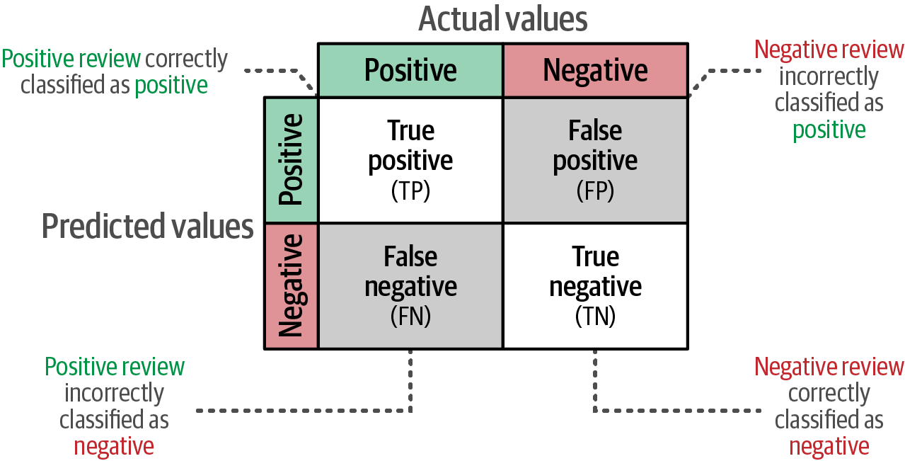
A confusion matrix visualizes the performance of a classification model by showing the counts of four prediction outcomes: True Positives, True Negatives, False Positives, and False Negatives, which serves as the basis for calculating various metrics to evaluate the model’s quality.
4.1.2. Embedding model
-
Without fine-tuning a representation model, a general-purpose embedding model can generate features that are then fed into a separate, trainable classifier (like logistic regression, which can be trained efficiently on a CPU), creating a two-step classification approach.
-
A major benefit of this separation is avoiding the costly fine-tuning of the embedding model, instead, a classifier, such as logistic regression, can be trained efficiently on the CPU.
from datasets import load_dataset

# load the well-known 'rotten_tomatoes' dataset for sentiment analysis
data = load_dataset("rotten_tomatoes")

# load the SentenceTransformer model for generating text embeddings
from sentence_transformers import SentenceTransformer
model = SentenceTransformer("sentence-transformers/all-mpnet-base-v2")

# convert the text data from the train and test splits into embeddings
train_embeddings = model.encode(data["train"]["text"], show_progress_bar=True)
test_embeddings = model.encode(data["test"]["text"], show_progress_bar=True)

from sklearn.linear_model import LogisticRegression

# train a logistic regression classifier on the generated training embeddings
#   initialize the logistic regression model with a random state for reproducibility
clf = LogisticRegression(random_state=42)
#   train the classifier using the training embeddings and their corresponding labels
clf.fit(train_embeddings, data["train"]["label"])

from sklearn.metrics import classification_report


def evaluate_performance(y_true, y_pred):
    '''Create and print the classification report comparing true and predicted labels'''
    performance = classification_report(
        y_true, y_pred, target_names=["Negative Review", "Positive Review"]
    )
    print(performance)


# predict the sentiment labels for the test embeddings using the trained classifier
y_pred = clf.predict(test_embeddings)

# evaluate the performance of the classifier on the test set
evaluate_performance(data["test"]["label"], y_pred)
precision recall f1-score support Negative Review 0.85 0.86 0.85 533 Positive Review 0.86 0.85 0.85 533 accuracy 0.85 1066 macro avg 0.85 0.85 0.85 1066 weighted avg 0.85 0.85 0.85 1066 -
Zero-shot classification can be used on unlabeled data by leveraging the model’s pre-existing knowledge to predict labels based solely on their definitions.
-
In zero-shot classification, without any labeled examples, the model determines the relationship between input text and predefined candidate labels.
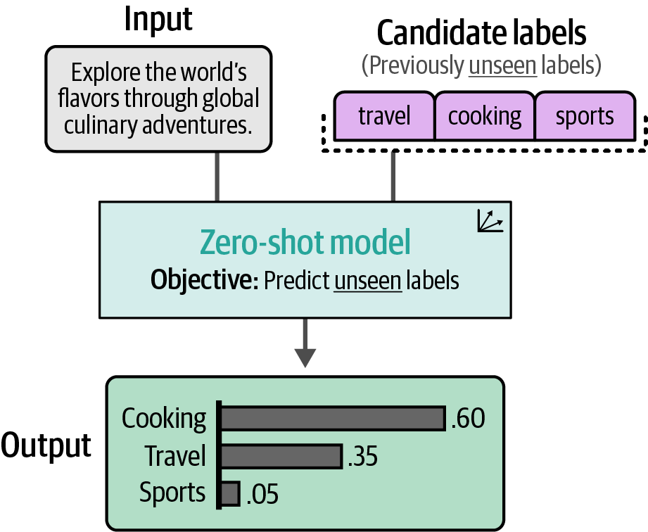 Figure 37. In zero-shot classification, we have no labeled data, only the labels them‐ selves. The zero-shot model decides how the input is related to the candidate labels.
 -
Zero-shot classification generates target labels without labeled data by describing and embedding labels (e.g., "negative movie review") and documents.
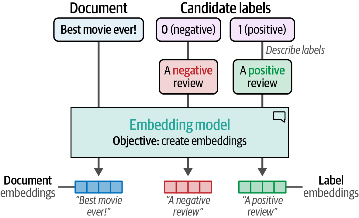 Figure 38. To embed the labels, we first need to give them a description, such as “a negative movie review.” This can then be embedded through sentence-transformers.
 -
To assign labels to documents in zero-shot classification, cosine similarity, representing the cosine of the angle between the embedding vectors, can be applied to document-label embedding pairs.
from datasets import load_dataset

# load the well-known 'rotten_tomatoes' dataset for sentiment analysis
data = load_dataset('rotten_tomatoes')

from sentence_transformers import SentenceTransformer

# load model
model = SentenceTransformer('sentence-transformers/all-mpnet-base-v2')

# convert text to embeddings
train_embeddings = model.encode(data['train']['text'], show_progress_bar=True)
test_embeddings = model.encode(data['test']['text'], show_progress_bar=True)

# create embeddings for our labels
label_embeddings = model.encode(['A negative review', 'A positive review'])

import numpy as np
from sklearn.metrics.pairwise import cosine_similarity
# find the best matching label for each document using cosine similarity
sim_matrix = cosine_similarity(test_embeddings, label_embeddings)
# get the index of the label with the highest similarity score for each test embedding
y_pred = np.argmax(sim_matrix, axis=1)

from sklearn.metrics import classification_report

def evaluate_performance(y_true, y_pred):
    '''Create and print the classification report comparing true and predicted labels'''
    performance = classification_report(
        y_true, y_pred, target_names=['Negative Review', 'Positive Review']
    )
    print(performance)

evaluate_performance(data['test']['label'], y_pred)
precision recall f1-score support Negative Review 0.78 0.77 0.78 533 Positive Review 0.77 0.79 0.78 533 accuracy 0.78 1066 macro avg 0.78 0.78 0.78 1066 weighted avg 0.78 0.78 0.78 1066From Wikipedia, the free encyclopedia
In data analysis, cosine similarity is a measure of similarity between two non-zero vectors defined in an inner product space. Cosine similarity is the cosine of the angle between the vectors; that is, it is the dot product of the vectors divided by the product of their lengths. It follows that the cosine similarity does not depend on the magnitudes of the vectors, but only on their angle. The cosine similarity always belongs to the interval
[−1, 1].
import numpy as np  # import the NumPy library for numerical operations

A = np.array([1, 2, 3])  # create a NumPy array named A
B = np.array([4, 5, 6])  # create a NumPy array named B

# calculate the cosine similarity using the formula: (A dot B) / (||A|| * ||B||)
dot_product = np.dot(A, B)  # calculate the dot product of A and B
norm_A = np.linalg.norm(A)  # calculate the Euclidean norm (magnitude) of A
norm_B = np.linalg.norm(B)  # calculate the Euclidean norm (magnitude) of B
cosine_similarity = dot_product / (norm_A * norm_B)  # calculate the cosine similarity

print(cosine_similarity)  # 0.9746318461970762
-
4.2. Generative Models
-
Text classification with generative language models (like GPT) involves feeding input text to the model and having it generate text as output, in contrast to task-specific models that directly output a class label.
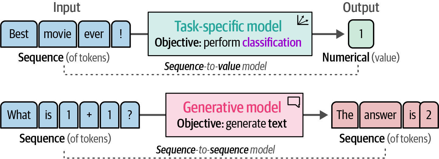 Figure 39. A task-specific model generates numerical values from sequences of tokens while a generative model generates sequences of tokens from sequences of tokens.
 -
Generative models are generally trained on a wide variety of tasks and usually don’t inherently know how to handle specific tasks like classifying a movie review without explicit instructions.
-
Prompt engineering is the skill of crafting effective instructions, or prompts, to guide generative AI models towards producing desired and high-quality outputs for specific tasks, like text classification, which often involves iterative refinement of these prompts based on the model’s responses.
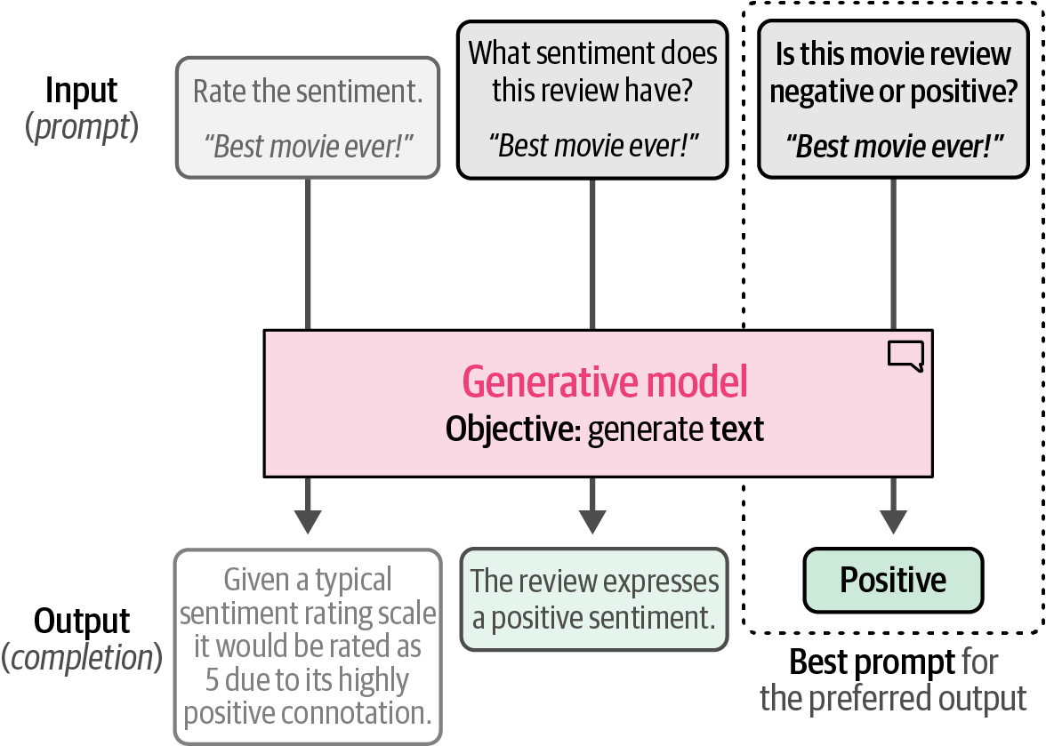 Figure 40. Prompt engineering allows prompts to be updated to improve the output generated by the model.
4.2.1. Text-to-Text Transfer Transformer
-
Text-to-Text Transfer Transformer or T5, like the original Transformer, is a generative encoder-decoder sequence-to-sequence model, contrasting with encoder-only BERT and decoder-only GPT.
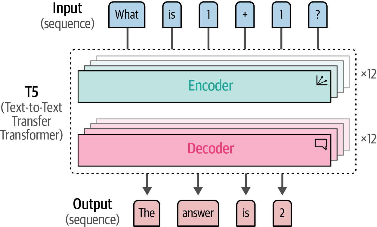 Figure 41. The T5 architecture is similar to the original Transformer model, a decoder- encoder architecture.
-
In the first step of training, namely pretraining, encoder-decoder models like T5 are initially trained with a masked language modeling objective that masks sets of tokens (or token spans), differing from BERT’s individual token masking approach.
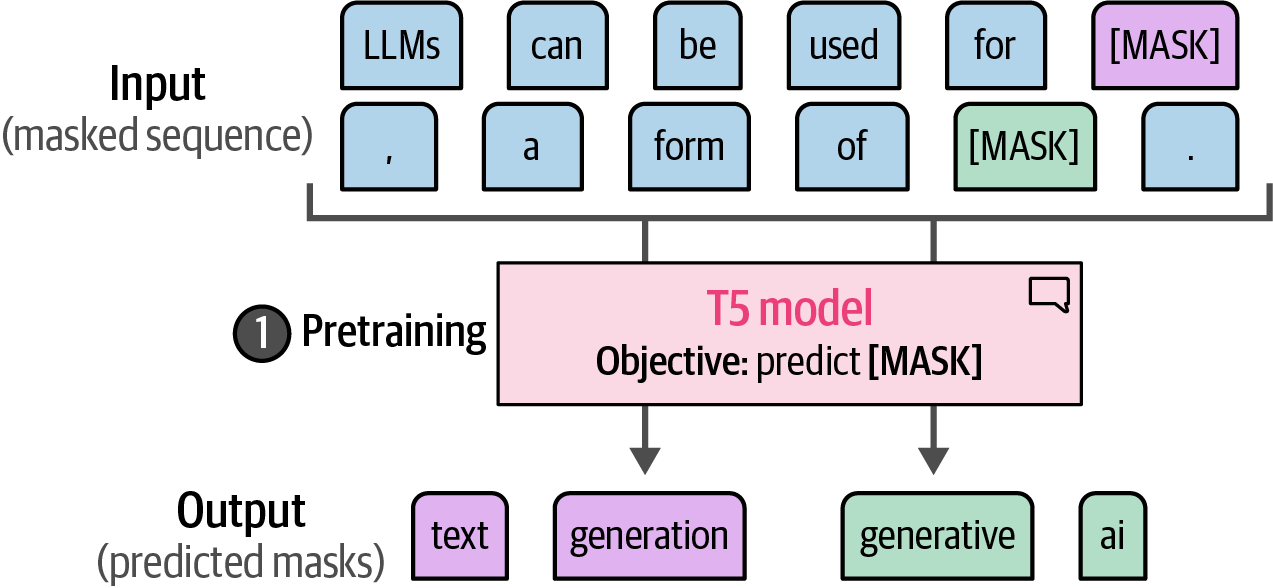 Figure 42. In the first step of training, namely pretraining, the T5 model needs to predict masks that could contain multiple tokens.
 -
In the second step of training, namely fine-tuning the base model, instead of fine-tuning the model for one specific task, each task is converted to a sequence-to-sequence task and trained simultaneously.
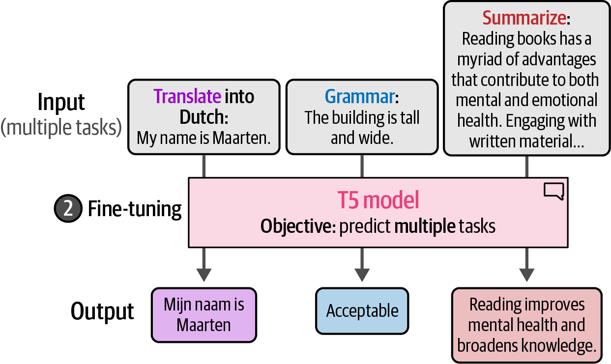 Figure 43. By converting specific tasks to textual instructions, the T5 model can be trained on a variety of tasks during fine-tuning.
-
from datasets import load_dataset

# load the well-known 'rotten_tomatoes' dataset for sentiment analysis
data = load_dataset('rotten_tomatoes')

import torch

# determine the device to use for computation (GPU if available, otherwise CPU)
dev = 'cuda' if torch.cuda.is_available() else 'cpu'

from transformers import pipeline

# specify the path to the pre-trained FLAN-T5-small model for text-to-text generation
model_path = 'google/flan-t5-small'
# load the pre-trained text-to-text generation model into a pipeline for easy inference
pipe = pipeline(
    'text2text-generation',
    model=model_path,
    device=dev,
)

# prepare our data by creating a prompt and combining it with the text
prompt = 'Is the following sentence positive or negative? '
# apply the prompt to each example in the dataset's 'text' column to create a new 't5' column
data = data.map(lambda example: {'t5': prompt + example['text']})
# data # uncomment to inspect the modified dataset

from tqdm import tqdm  # for progress bar during inference
from transformers.pipelines.pt_utils import (
    KeyDataset,
)  # utility to feed data to the pipeline

# Run inference
y_pred = []
# iterate through the test dataset using the pipeline for text generation
for output in tqdm(
    pipe(KeyDataset(data['test'], 't5')), total=len(data['test'])
):
    # extract the generated text from the pipeline's output
    text = output[0]['generated_text']
    # classify the generated text as 0 (negative) if it equals 'negative', otherwise 1 (positive)
    y_pred.append(0 if text == 'negative' else 1)

from sklearn.metrics import classification_report


def evaluate_performance(y_true, y_pred):
    '''Create and print the classification report comparing true and predicted labels'''
    performance = classification_report(
        y_true, y_pred, target_names=['Negative Review', 'Positive Review']
    )
    print(performance)


# evaluate the performance of the model by comparing the true labels with the predicted labels
evaluate_performance(data['test']['label'], y_pred)
precision recall f1-score support
Negative Review 0.83 0.85 0.84 533
Positive Review 0.85 0.83 0.84 533
accuracy 0.84 1066
macro avg 0.84 0.84 0.84 1066
weighted avg 0.84 0.84 0.84 10664.2.2. ChatGPT for Classification
OpenAI shared an overview of the training procedure that involved an important component, namely preference tuning.
-
OpenAI first manually created the desired output to an input prompt (instruction data) and used that data to create a first variant of its model.
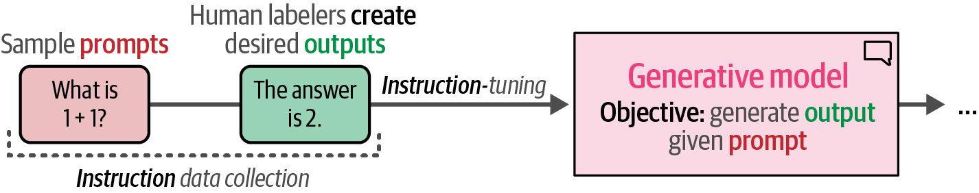 Figure 44. Manually labeled data consisting of an instruction (prompt) and output was used to perform fine-tuning (instruction-tuning).
 -
OpenAI used the resulting model to generate multiple outputs that were manually ranked from best to worst.
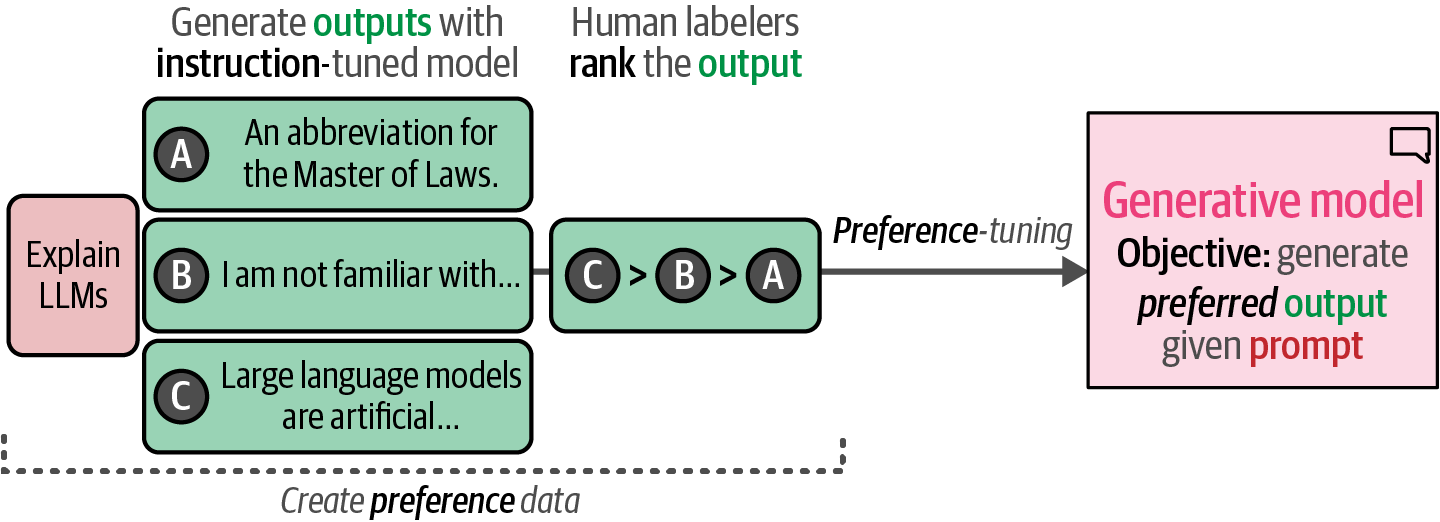 Figure 45. Manually ranked preference data was used to generate the final model, ChatGPT.
import openai

# create client for interacting with OpenAI API
client = openai.OpenAI(api_key='YOUR_KEY_HERE')


def chatgpt_generation(prompt, document, model='gpt-3.5-turbo-0125'):
    '''Generate an output based on a prompt and an input document using ChatGPT.'''
    # define the message structure for the OpenAI API
    messages = [
        {'role': 'system', 'content': 'You are a helpful assistant.'},
        {'role': 'user', 'content': prompt.replace('[DOCUMENT]', document)},
    ]
    # call the OpenAI Chat Completions API to get a response
    chat_completion = client.chat.completions.create(
        messages=messages, model=model, temperature=0 # temperature=0 for deterministic output
    )
    # return the content of the first choice's message
    return chat_completion.choices[0].message.content


# define a prompt template as a base for sentiment classification
prompt = '''Predict whether the following document is a positive or negative
movie review:
[DOCUMENT]
If it is positive return 1 and if it is negative return 0. Do not give any
other answers.
'''

# predict the target for a single document using GPT
document = 'unpretentious , charming , quirky , original'
chatgpt_generation(prompt, document)


from datasets import load_dataset

# load the well-known 'rotten_tomatoes' dataset for sentiment analysis
data = load_dataset('rotten_tomatoes')

from tqdm import tqdm

# generate predictions for all documents in the test set
predictions = [
    chatgpt_generation(prompt, doc) for doc in tqdm(data['test']['text'])
]

# convert the string predictions ('0' or '1') to integers
y_pred = [int(pred) for pred in predictions]

from sklearn.metrics import classification_report


def evaluate_performance(y_true, y_pred):
    '''Create and print the classification report comparing true and predicted labels'''
    performance = classification_report(
        y_true, y_pred, target_names=['Negative Review', 'Positive Review']
    )
    print(performance)


# evaluate the performance of ChatGPT on the test set
evaluate_performance(data['test']['label'], y_pred)
5. Text Clustering and Topic Modeling
Although supervised techniques, such as classification, have reigned supreme over the last few years in the industry, the potential of unsupervised techniques such as text clustering cannot be understated.
-
Text clustering aims to group similar texts based on their semantic content, meaning, and relationships.
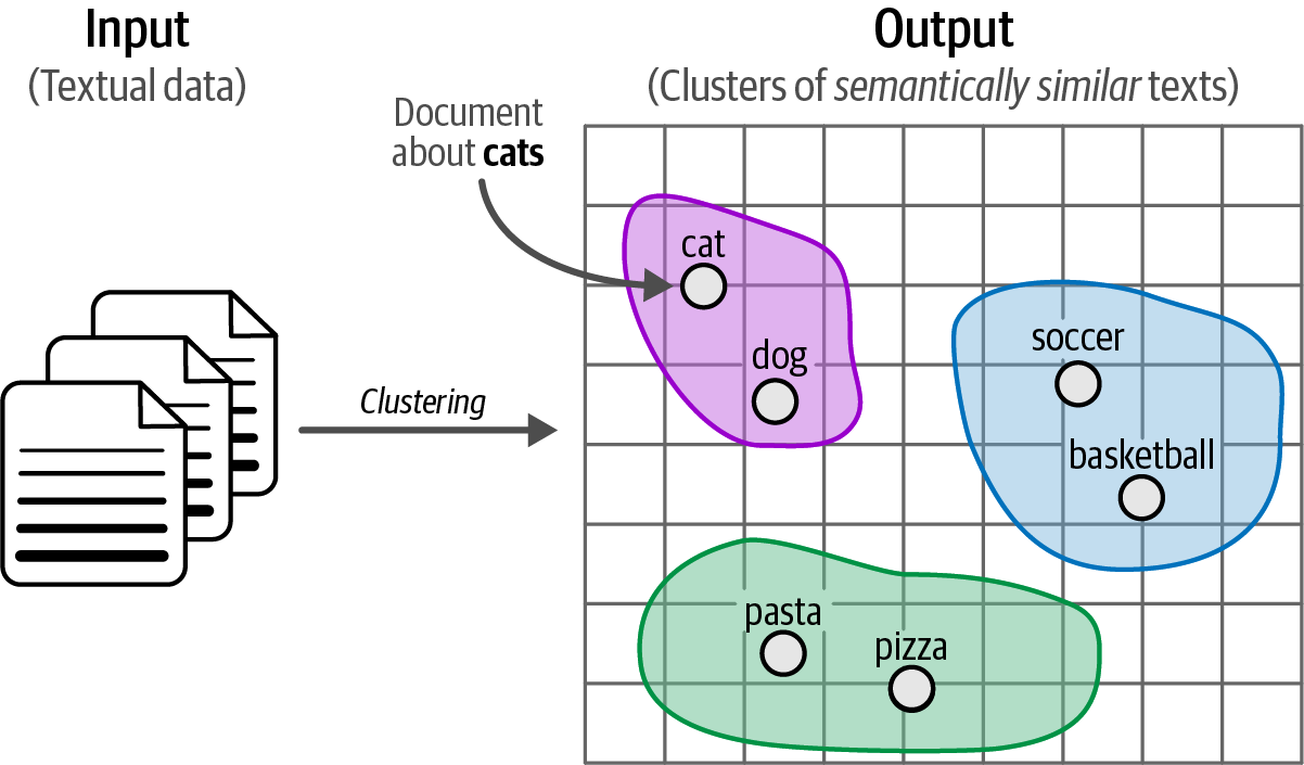 Figure 46. Clustering unstructured textual data.
 -
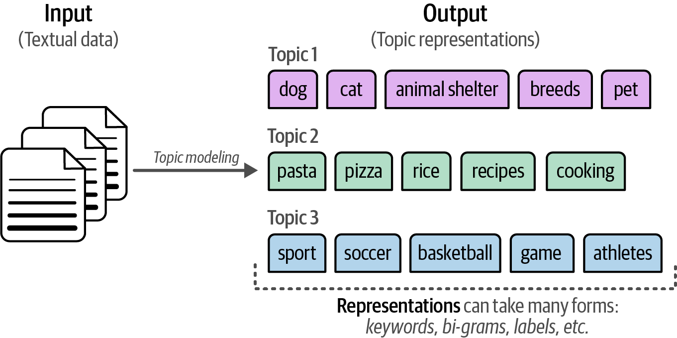
Text clustering is also applied in topic modeling to uncover abstract topics within large textual datasets.
 Figure 47. Topic modeling is a way to give meaning to clusters of textual documents.
5.1. ArXiv’s Articles: Computation and Language
ArXiv is an open-access platform for scholarly articles, mostly in the fields of computer science, mathematics, and physics.
from datasets import load_dataset

# load the 'arxiv_nlp' dataset from Hugging Face Datasets library
dataset = load_dataset("maartengr/arxiv_nlp")["train"]

# extract metadata
abstracts = dataset["Abstracts"]
titles = dataset["Titles"]
5.2. A Common Pipeline for Text Clustering
Text clustering enables the discovery of both known and unknown data patterns, providing an intuitive understanding of tasks like classification and their complexity, making it valuable beyond just exploratory data analysis.
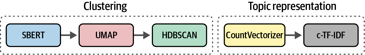
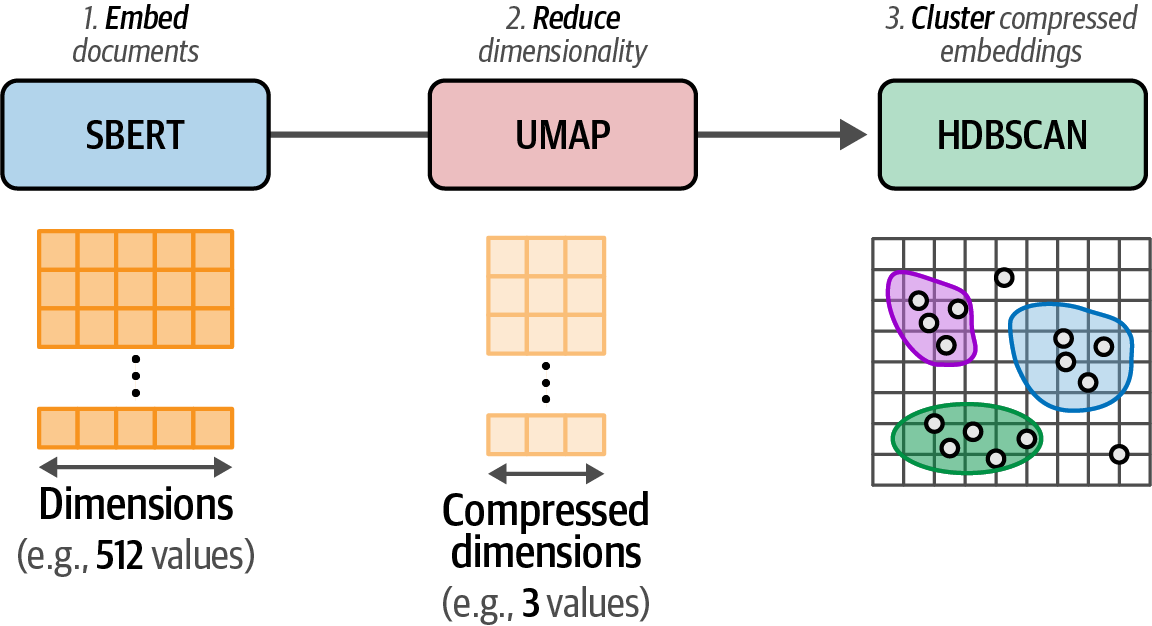
Although there are many methods for text clustering, from graph-based neural networks to centroid-based clustering techniques, a common pipeline that has gained popularity involves three steps and algorithms:
-
Convert the input documents to embeddings with an embedding model.
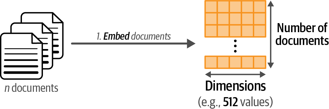 Figure 48. Step 1: We convert documents to embeddings using an embedding model.
 -
Reduce the dimensionality of embeddings with a dimensionality reduction model.
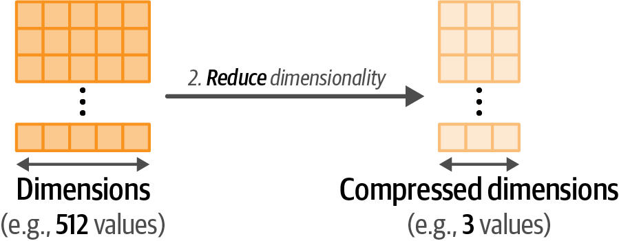 Figure 49. Step 2: The embeddings are reduced to a lower-dimensional space using dimensionality reduction.
 -
Find groups of semantically similar documents with a cluster model.
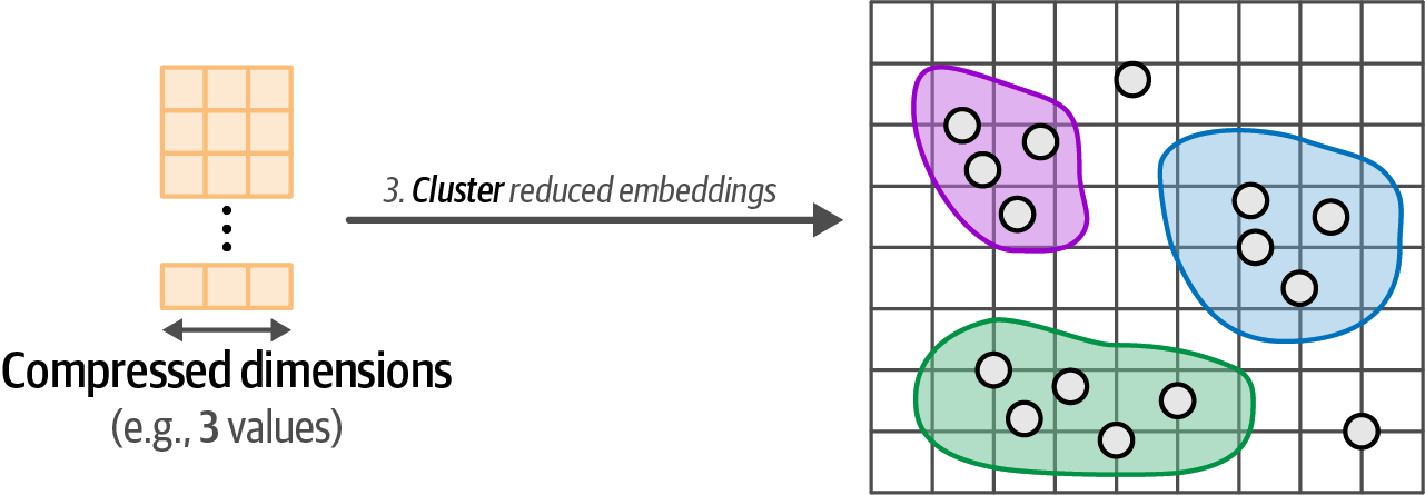 Figure 50. Step 3: We cluster the documents using the embeddings with reduced dimensionality.
5.2.1. Embedding Documents
from sentence_transformers import SentenceTransformer

# create an embedding model using a pre-trained Sentence Transformer model
embedding_model = SentenceTransformer('thenlper/gte-small') (1)

# generate embeddings for each abstract in the 'abstracts' list
embeddings = embedding_model.encode(abstracts, show_progress_bar=True)

# check the dimensions (shape) of the resulting embeddings
embeddings.shape # (44949, 384) (2)
| 1 | The thenlper/gte-small model is a more recent model that outperforms the previous model on clustering tasks and due to its small size is even faster for inference. |
| 2 | The embeddings.shape of (44949, 384) shows that there are 44,949 abstract embeddings, each with a dimensionality of 384. |
5.2.2. Reducing the Dimensionality of Embeddings
-
Reducing the dimensionality of embeddings is essential before clustering high-dimensional data to simplify the representation and enhance clustering effectiveness.
-
Dimensionality reduction is a compression technique and that the underlying algorithm is not arbitrarily removing dimensions.
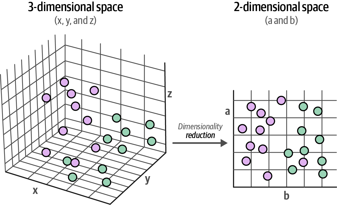 Figure 51. Dimensionality reduction allows data in high-dimensional space to be compressed to a lower-dimensional representation.
 -
Well-known methods for dimensionality reduction are Principal Component Analysis (PCA) and Uniform Manifold Approximation and Projection (UMAP).
from umap import UMAP

# reduce the input embeddings from 384 dimensions to 5 dimensions using UMAP
umap_model = UMAP(
    # generally, values between 5 and 10 work well to capture high-dimensional global structures.
    n_components=5,   # the number of dimensions to reduce to
    min_dist=0.0,     # the effective minimum distance between embedded points
    metric='cosine',  # the metric to use to compute distances in high dimensional space
    random_state=42,  # for reproducibility of the embedding
)
# fit and then transform the embeddings to the lower-dimensional space
reduced_embeddings = umap_model.fit_transform(embeddings)
5.2.3. Cluster the Reduced Embeddings
-
While k-means, a centroid-based algorithm needing a predefined number of clusters, is common, density-based algorithms are preferable when the number of clusters is unknown as they automatically determine the clusters and don’t require all data points to belong to one.
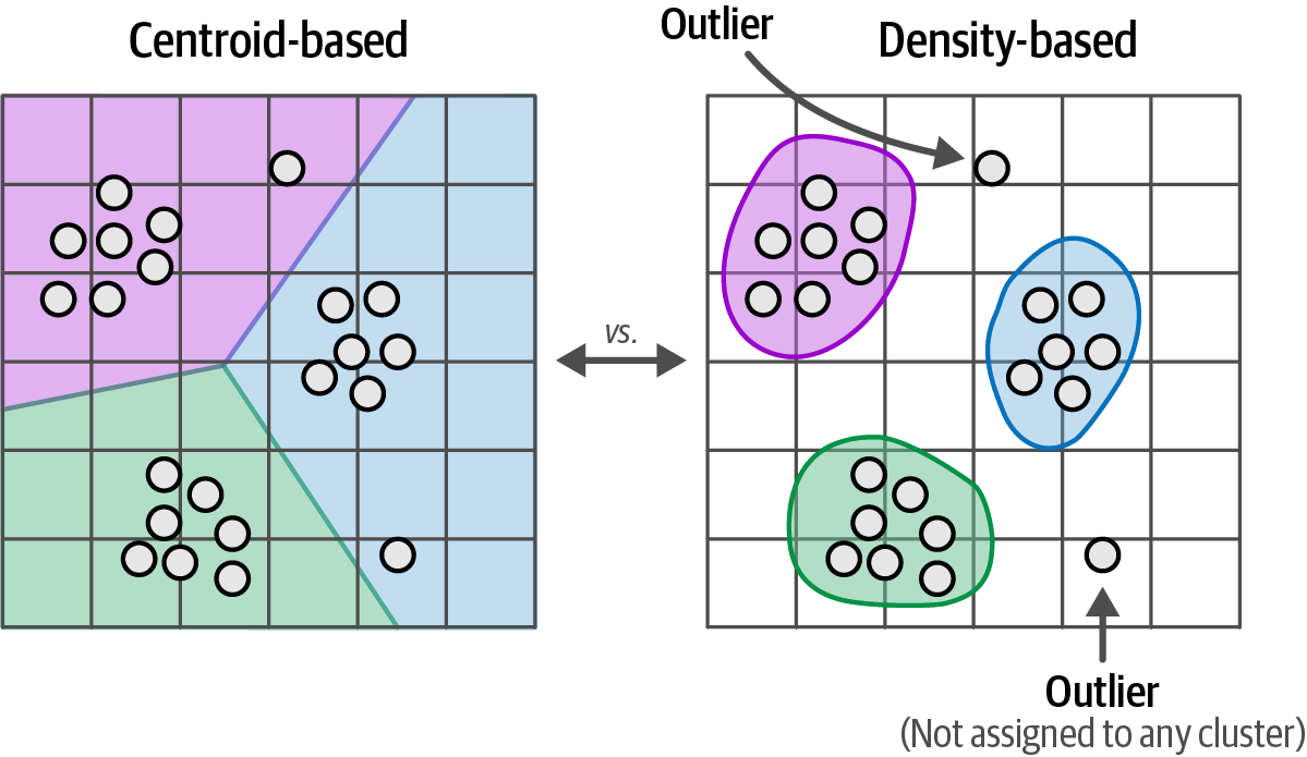 Figure 52. The clustering algorithm not only impacts how clusters are generated but also how they are viewed.
 -
A common density-based model is Hierarchical Density-Based Spatial Clustering of Applications with Noise (HDBSCAN).
from hdbscan import HDBSCAN

# initialize and fit the HDBSCAN clustering model
hdbscan_model = HDBSCAN(
    # the minimum number of samples in a group for it to be considered a cluster
    min_cluster_size=50,
    # the metric to use when calculating pairwise distances between data points
    metric='euclidean',
    # the method used to select clusters from the hierarchy ('eom' stands for Excess of Mass)
    cluster_selection_method='eom'
).fit(reduced_embeddings) # fit the HDBSCAN model to the reduced dimensionality embeddings
# extract the cluster labels assigned to each data point (-1 indicates noise)
clusters = hdbscan_model.labels_
# How many clusters did we generate? (excluding the noise cluster labeled -1)
num_clusters = len(set(clusters)) - (1 if -1 in clusters else 0)
5.2.4. Inspecting the Clusters
-
To inspect each cluster manually and explore the assigned documents to get an understanding of its content.
import numpy as np # print first three documents in cluster 0 cluster = 0 for index in np.where(clusters == cluster)[0][:3]: print(abstracts[index][:300] + "... \n") -
To visualize clustering approximation results without manual review, further reduce document embeddings to two dimensions for plotting on an 2D plane.
import pandas as pd from umap import UMAP import matplotlib.pyplot as plt # reduce 384-dimensional embeddings to two dimensions for easier visualization reduced_embeddings = UMAP( n_components=2, min_dist=0.0, metric="cosine", random_state=42, ).fit_transform(embeddings) # create dataframe df = pd.DataFrame(reduced_embeddings, columns=["x", "y"]) df["title"] = titles df["cluster"] = [str(c) for c in clusters] # select outliers (cluster -1) and non-outliers (clusters) to_plot = df.loc[df.cluster != "-1", :] outliers = df.loc[df.cluster == "-1", :] # plot outliers and non-outliers separately plt.scatter(outliers.x, outliers.y, alpha=0.05, s=2, c="grey", label="Outliers") plt.scatter( to_plot.x, to_plot.y, c=to_plot.cluster.astype(int), alpha=0.6, s=2, cmap="tab20b", label="Clusters", ) plt.axis("off") plt.legend() # Add a legend to distinguish outliers and clusters plt.title("Visualization of Clustered Abstracts") # Add a title for context plt.show()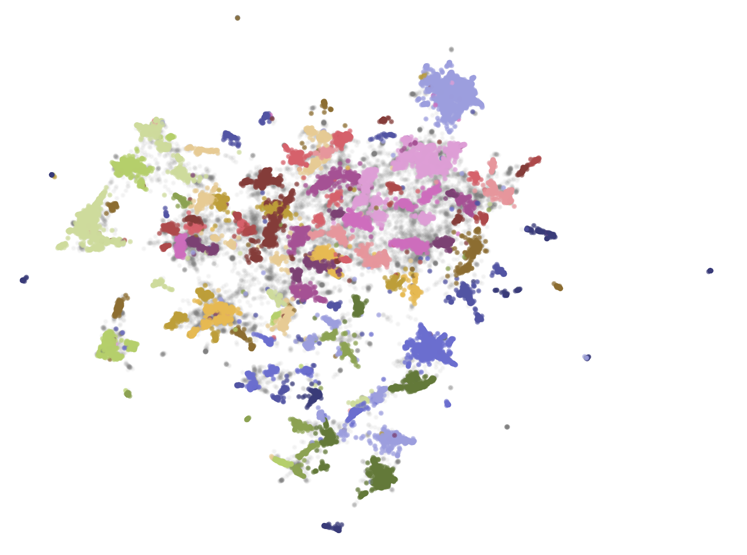 Figure 53. The generated clusters (colored) and outliers (gray) are represented as a 2D visualization.
5.3. From Text Clustering to Topic Modeling
Text clustering is a powerful tool for finding structure among large collections of documents, whereas topic modeling is the process of discovering underlying themes or latent topics within a collection of textual data, which typically involves finding a set of keywords or phrases that best represent and capture the meaning of the topic.
5.3.1. BERTopic: A Modular Topic Modeling Framework
BERTopic is a topic modeling technique that leverages clusters of semantically similar texts to extract various types of topic representations.
-
First, similar to text clustering, it embeds documents, reduces their dimensionality, and then clusters these embeddings to group semantically similar texts. .The first part of BERTopic’s pipeline is to create clusters of semantically similar documents.
-
Second, it models word distributions using a bag-of-words approach, counting word frequencies within documents to help extract the most frequent terms.
The bag-of-words approach does exactly what its name implies: it counts the number of times each word appears in a document, which can then be used to extract the most frequent words within that document.
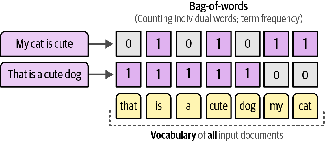 Figure 56. A bag-of-words counts the number of times each word appears inside a document.
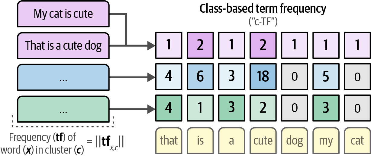 Figure 57. Generating c-TF by counting the frequency of words per cluster instead of per document.
6. Prompt Engineering
Prompt engineering is the art and science of crafting effective prompts to guide large language models (LLMs) and other generative AI systems to produce desired and high-quality outputs. It involves understanding how these models interpret and respond to different phrasings, instructions, and contexts within a prompt to achieve specific goals, such as generating creative text, answering questions accurately, or performing tasks effectively.
6.1. Using Text Generation Models
import torch
from transformers import AutoModelForCausalLM, AutoTokenizer, pipeline

# determine the device
dev = 'cuda' if torch.cuda.is_available() else 'cpu'

# load model and tokenizer
model_path = 'microsoft/Phi-4-mini-instruct'
model = AutoModelForCausalLM.from_pretrained(
    model_path,
    device_map=dev,
    torch_dtype='auto',
    trust_remote_code=True,
)
tokenizer = AutoTokenizer.from_pretrained(model_path)

# create a pipeline
pipe = pipeline(
    'text-generation',
    model=model,
    tokenizer=tokenizer,
    return_full_text=False,
    max_new_tokens=500,
    do_sample=False,
)

# prompt
messages = [{'role': 'user', 'content': 'Create a funny joke about chickens.'}]

# generate the output
output = pipe(messages)
print(output[0]['generated_text'])
6.1.1. Prompt Template
-
Under the hood,
transformers.pipelinefirst converts the messages into a specific prompt template which was used during the training of the model.# apply prompt template prompt = pipe.tokenizer.apply_chat_template(messages, tokenize=False) print(prompt)<s><|user|> Create a funny joke about chickens.<|end|> <|assistant|>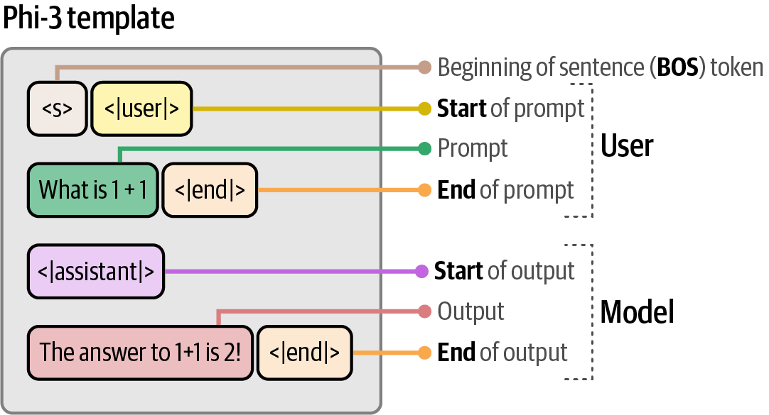 Figure 58. The template Phi-3 expects when interacting with the model.
6.1.2. Controlling Model Output
-
Each time an LLM needs to generate a token, it assigns a likelihood number to each possible token to generate different responses for the exact same prompt.
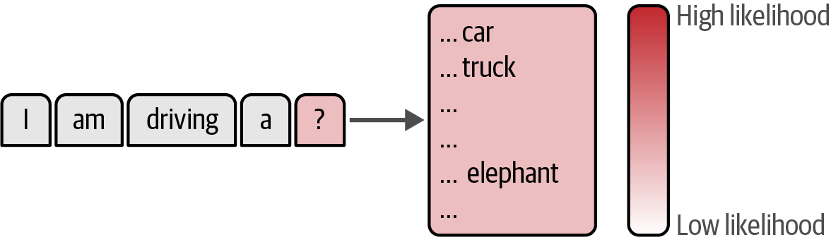 Figure 59. The model chooses the next token to generate based on their likelihood scores.
 -
The
temperaturecontrols the randomness or creativity of the text generated; a higher temperature increases creativity by making less probable tokens more likely, while a temperature of0results in deterministic output by always selecting the most probable token.# using a high temperature output = pipe(messages, do_sample=True, temperature=1) print(output[0]["generated_text"])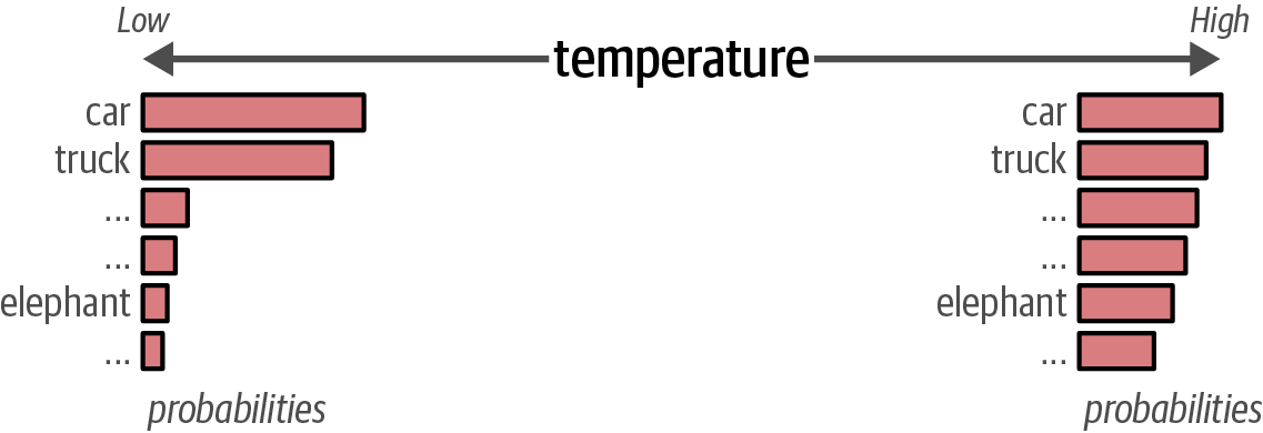 Figure 60. A higher temperature increases the likelihood that less probable tokens are generated and vice versa.
 -
The
top-p, or nucleus sampling, is a technique that controls the subset of tokens (the nucleus) an LLM considers for generation by including tokens until their cumulative probability reaches a specified threshold.For instance, if
top_pis set to0.1, the model will consider tokens until their cumulative probability reaches 10%, and iftop_pis set to1, all tokens will be considered.# using a high top_p output = pipe(messages, do_sample=True, top_p=1) print(output[0]["generated_text"])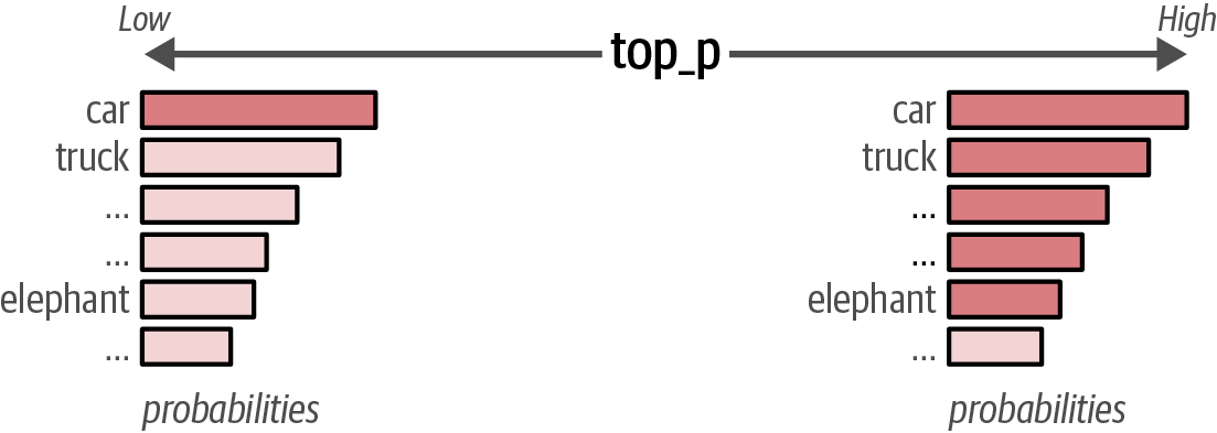 Figure 61. A higher top_p increases the number of tokens that can be selected to generate and vice versa.
 -
The
top_kparameter directly limits the number of most probable tokens an LLM considers; setting it to 100 restricts the selection to only the top 100 tokens.Table 1. Use case examples when selecting values for temperature and top_p. Example use case temperature top_p Description Brainstorming session
High
High
High randomness with large pool of potential tokens. The results will be highly diverse, often leading to very creative and unexpected results.
Email generation
Low
Low
Deterministic output with high probable predicted tokens. This results in predictable, focused, and conservative outputs.
Creative writing
High
Low
High randomness with a small pool of potential tokens. This combination produces creative outputs but still remains coherent.
Translation
Low
High
Deterministic output with high probable predicted tokens. Produces coherent output with a wider range of vocabulary, leading to outputs with linguistic variety.
6.2. Prompt Engineering
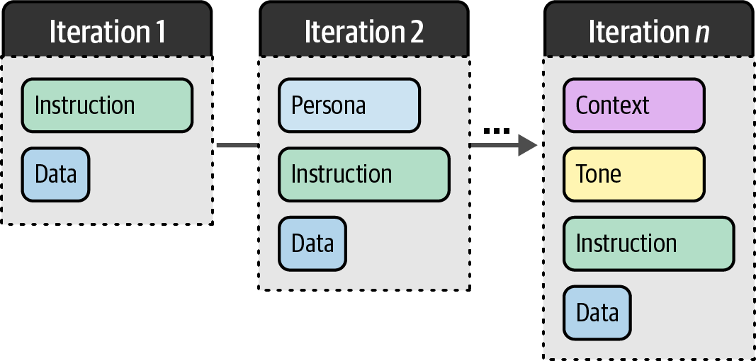
Prompt engineering is the iterative process of designing effective prompts, including questions, statements, or instructions, to elicit useful and relevant outputs from LLMs through experimentation and optimization.
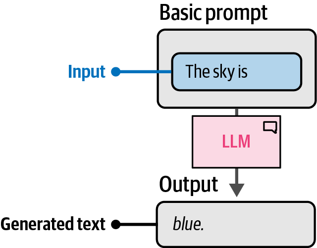
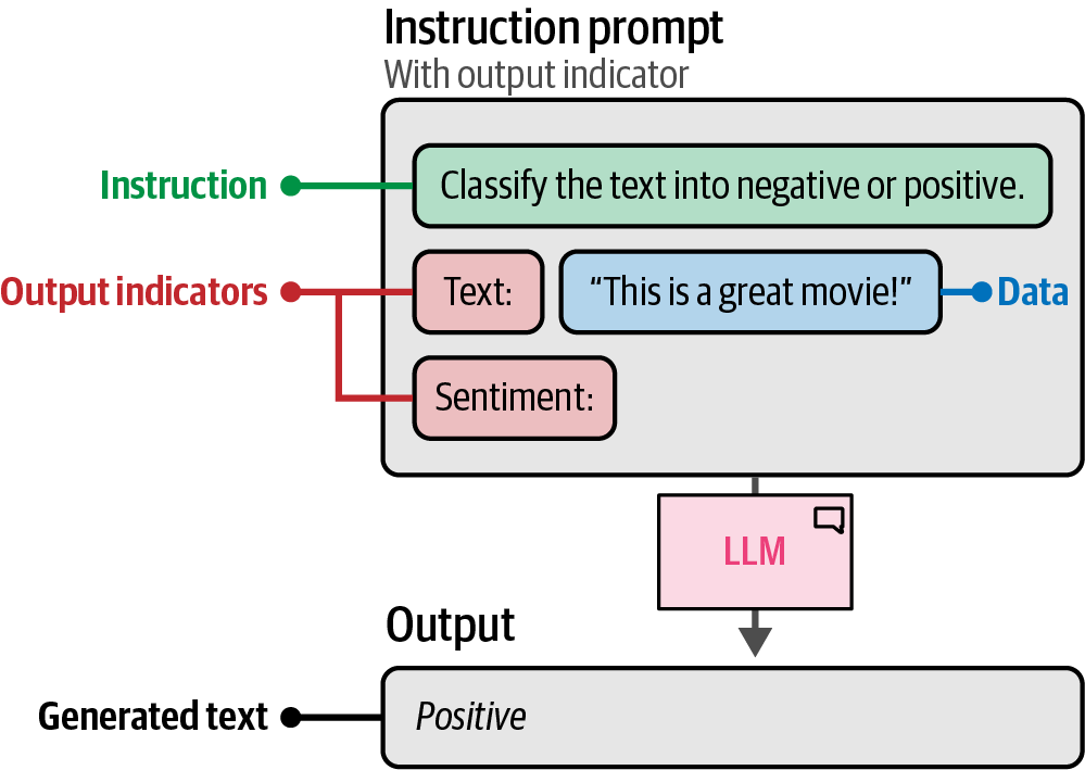
A prompt is the input provided to a large language model to elicit a desired response, which generally consists of multiple components such as instructions, data, and output indicators, and can be as complex as needed.
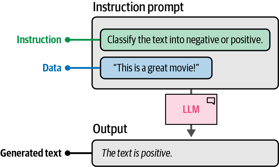
6.3. Instruction-Based Prompting
Instruction-based prompting is a method of prompting where the primary goal is to have the LLM answer a specific question or resolve a certain task by providing it with specific instructions.
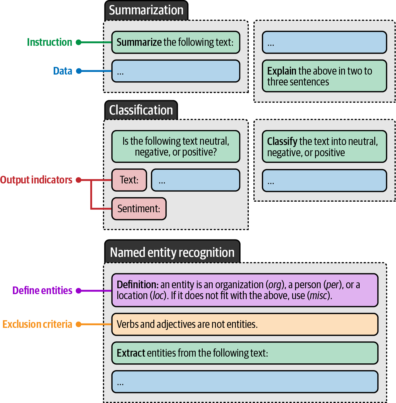
Each of these tasks requires different prompting formats and more specifically, asking different questions of the LLM. A non-exhaustive list of the prompting techniques includes:
-
Specificity
Accurately describe the desired output, for example, instead of "Write a product description," ask "Write a product description in under two sentences using a formal tone."
Specificity is arguably the most important aspect; by restricting and specifying what the model should generate, there is a smaller chance of it generating something unrelated to a use case.
-
Hallucination
LLMs may generate incorrect information confidently, which is referred to as hallucination.
To reduce its impact, ask the LLM to only generate an answer if it knows the answer, and to respond with "I don’t know" if it does not know the answer.
-
Order
Either begin or end the prompt with the instruction.
Especially with long prompts, information in the middle is often forgotten.
LLMs tend to focus on information either at the beginning of a prompt (primacy effect) or the end of a prompt (recency effect).
6.4. Advanced Prompt Engineering
While creating a good prompt might initially seem straightforward—just ask a specific question, be accurate, and add examples—prompting can quickly become complex and is often an underestimated aspect of effectively using LLMs.
6.4.1. Prompt Components
A prompt generally consists of multiple components, such as instruction, data, and output indicators, and other advanced components that can quickly make a prompt quite complex.
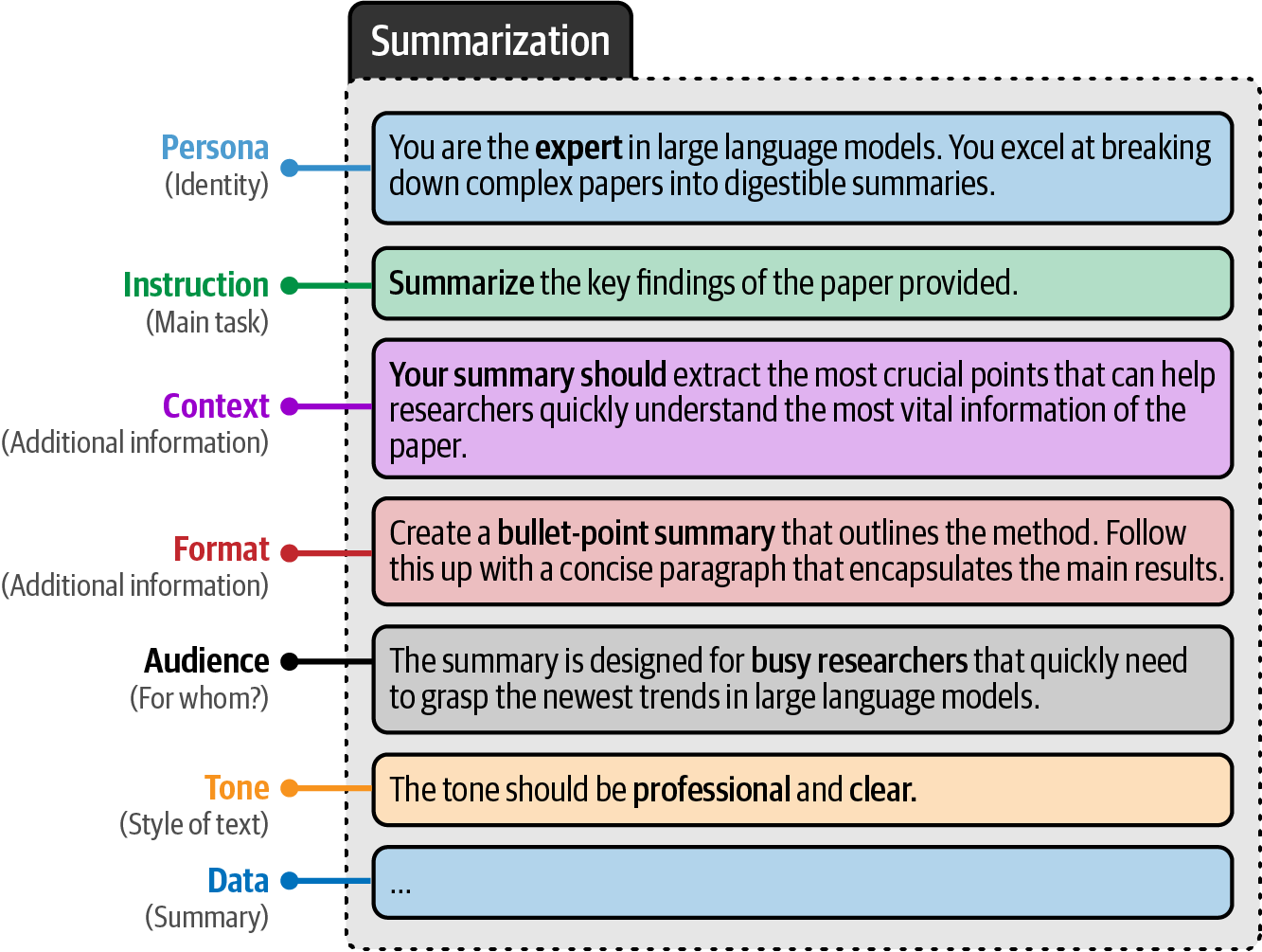
# prompt components
persona = 'You are an expert in Large Language models. You excel at breaking down complex papers into digestible summaries.\n'
instruction = 'Summarize the key findings of the paper provided.\n'
context = 'Your summary should extract the most crucial points that can help researchers quickly understand the most vital information of the paper.\n'
data_format = 'Create a bullet-point summary that outlines the method. Follow this up with a concise paragraph that encapsulates the main results.\n'
audience = 'The summary is designed for busy researchers that quickly need to grasp the newest trends in Large Language Models.\n'
tone = 'The tone should be professional and clear.\n'
text = 'MY TEXT TO SUMMARIZE'
data = f'Text to summarize: {text}'

# the full prompt - remove and add pieces to view its impact on the generated output
query = persona + instruction + context + data_format + audience + tone + data
6.4.2. In-Context Learning: Providing Examples
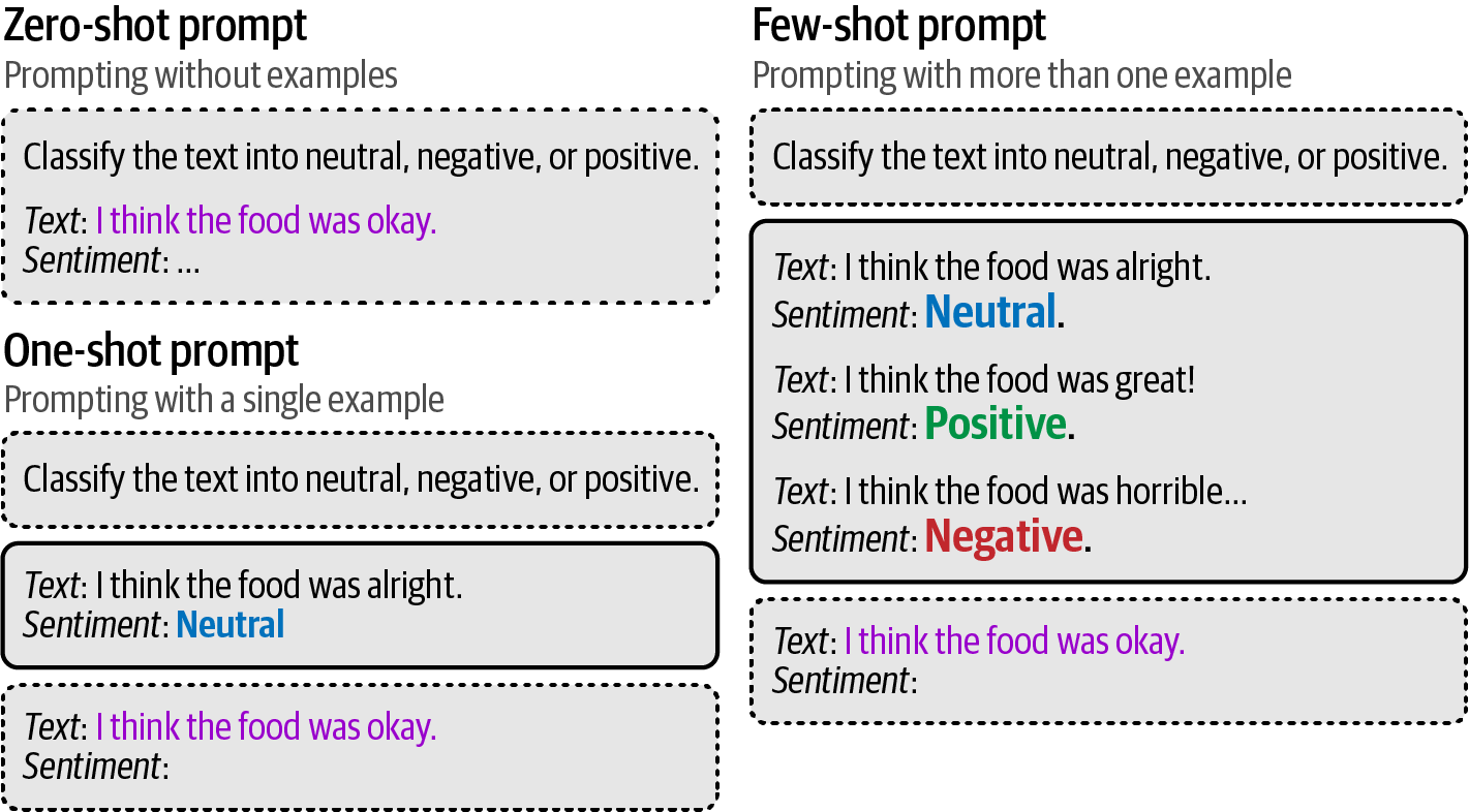
In-context learning (ICL) is a prompting technique that demonstrates the desired task to an LLM through direct examples, rather than solely describing it to provide the model with context to learn from within the prompt.
Zero-shot prompting does not leverage examples, one-shot prompts use a single example, and few-shot prompts use two or more examples.
# use a single example of using the made-up word in a sentence
one_shot_prompt = [
    {
        'role': 'user',
        'content': 'A \'Gigamuru\' is a type of Japanese musical instrument. An example of a sentence that uses the word Gigamuru is:',
    },
    {
        'role': 'assistant',
        'content': 'I have a Gigamuru that my uncle gave me as a gift. I love to play it at home.',
    },
    {
        'role': 'user',
        'content': 'To \'screeg\' something is to swing a sword at it. An example of a sentence that uses the word screeg is:',
    },
]
print(tokenizer.apply_chat_template(one_shot_prompt, tokenize=False))
<|user|>A 'Gigamuru' is a type of Japanese musical instrument. An example of a sentence that uses the word Gigamuru is:<|end|><|assistant|>I have a Gigamuru that my uncle gave me as a gift. I love to play it at home.<|end|><|user|>To 'screeg' something is to swing a sword at it. An example of a sentence that uses the word screeg is:<|end|><|endoftext|># generate the output
outputs = pipe(one_shot_prompt)
print(outputs[0]["generated_text"])In the medieval fantasy novel, the knight would screeg his enemies with his gleaming sword.6.4.3. Chain Prompting: Breaking up the Problem
Prompt chaining is a technique that addresses complex tasks by breaking them down across multiple prompts, where the output of one prompt serves as the input for the subsequent prompt, creating a sequence of interactions that collectively solve the problem.
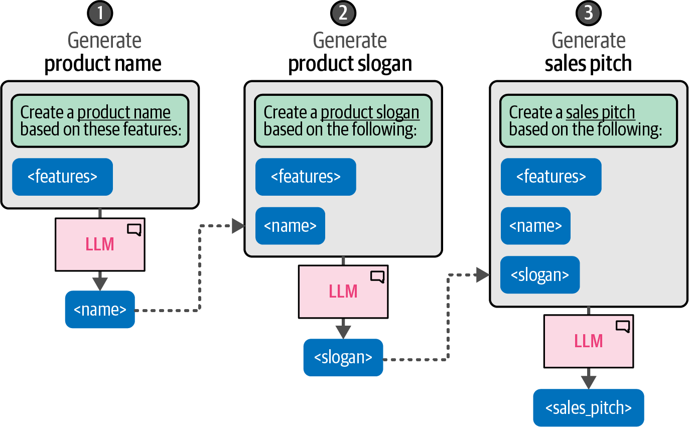
# create name and slogan for a product
product_prompt = [
    {
        "role": "user",
        "content": "Create a name and slogan for a chatbot that leverages LLMs.",
    }
]
outputs = pipe(product_prompt)
product_description = outputs[0]["generated_text"]
print(product_description)

# based on a name and slogan for a product, generate a sales pitch
sales_prompt = [
    {
        "role": "user",
        "content": f"Generate a very short sales pitch for the following product: '{product_description}'",
    }
]
outputs = pipe(sales_prompt)
sales_pitch = outputs[0]["generated_text"]
print(sales_pitch)
Name: LexiBot
Slogan: "Unlock the Power of Language with LexiBot – Your AI Conversation Partner!"
Discover the future of communication with LexiBot – your AI conversation partner. Say goodbye to language barriers and hello to seamless, intelligent interactions. LexiBot is here to unlock the power of language, making every conversation more engaging and productive. Embrace the power of AI with LexiBot today!6.5. Reasoning with Generative Models
Reasoning is a core component of human intelligence and is often compared to the emergent behavior of LLMs that often resembles reasoning (through memorization of training data and pattern matching, rather than true reasoning).
Human reasoning can be broadly categorized into two systems.
-
System 1 thinking represents an automatic, intuitive, and near-instantaneous process, which shares similarities with generative models that automatically generate tokens without any self-reflective behavior.
-
System 2 thinking, in contrast, is a conscious, slow, and logical process, akin to brainstorming and self-reflection.
The system 2 way of thinking, which tends to produce more thoughtful responses than system 1 thinking, would be emulated by giving a generative model the ability to mimic a form of self-reflection.
6.5.1. Chain-of-Thought: Think Before Answering
Chain-of-thought (CoT) prompting is a technique that allows large language models (LLMs) to solve a problem as a series of intermediate steps ("thoughts") before giving a final answer.
-
Although chain-of-thought is a great method for enhancing the output of a generative model, it does require one or more examples of reasoning in the prompt, which the user might not have access to.
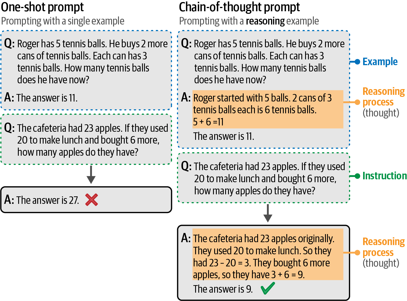 Figure 70. Chain-of-thought prompting uses reasoning examples to persuade the generative model to use reasoning in its answer.
# answering with chain-of-thought
cot_prompt = [
    {
        "role": "user",
        "content": "Roger has 5 tennis balls. He buys 2 more cans of tennis balls. Each can has 3 tennis balls. How many tennis balls does he have now?",
    },
    {
        "role": "assistant",
        "content": "Roger started with 5 balls. 2 cans of 3 tennis balls each is 6 tennis balls. 5 + 6 = 11. The answer is 11.",
    },
    {
        "role": "user",
        "content": "The cafeteria had 23 apples. If they used 20 to make lunch and bought 6 more, how many apples do they have?",
    },
]

# generate the output
outputs = pipe(cot_prompt)
print(outputs[0]["generated_text"])
The cafeteria started with 23 apples. They used 20, so they had 23 - 20 = 3 apples left. Then they bought 6 more, so they now have 3 + 6 = 9 apples. The answer is 9. -
Instead of providing examples, zero-shot chain-of-thought allows a generative model to provide reasoning without explicit examples by directly prompting it for its thought process.
Although the prompt “Let’s think step by step” can improve the output, you are not constrained by this exact formulation. Alterna‐ tives exist like “Take a deep breath and think step-by-step” and “Let’s work through this problem step-by-step.”
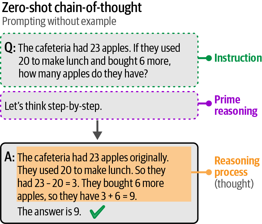 Figure 71. Chain-of-thought prompting without using examples. Instead, it uses the phrase “Let’s think step-by-step” to prime reasoning in its answer.
# zero-shot chain-of-thought prompt
zeroshot_cot_prompt = [
    {
        "role": "user",
        "content": "The cafeteria had 23 apples. If they used 20 to make lunch and bought 6 more, how many apples do they have? Let's think step-by-step.",
    }
]

# generate the output
outputs = pipe(zeroshot_cot_prompt)
print(outputs[0]["generated_text"])
Sure, let's break it down step-by-step: 1. The cafeteria starts with 23 apples. 2. They use 20 apples to make lunch. 3. After using 20 apples, they have: 23 apples - 20 apples = 3 apples left. 4. They then buy 6 more apples. 5. Adding the 6 new apples to the 3 apples they have left: 3 apples + 6 apples = 9 apples. So, the cafeteria now has 9 apples.
6.5.2. Self-Consistency: Sampling Outputs
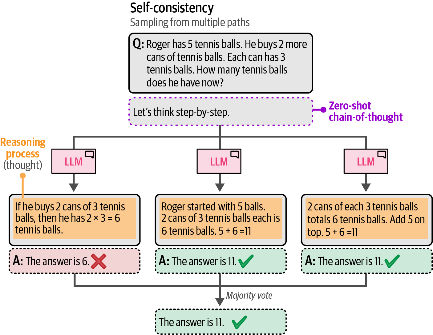
Self-consistency is a technique that reduces randomness in generative models by prompting them multiple times with the same input, using varied sampling parameters like temperature and top_p to enhance diversity, and selecting the majority result as the final answer for robustness.
# zero-shot chain-of-thought prompt
zeroshot_cot_prompt = [
    {
        "role": "user",
        "content": "The cafeteria had 23 apples. If they used 20 to make lunch and bought 6 more, how many apples do they have? Let's think step-by-step.",
    }
]

# self-consistency settings
num_samples = 3
temperature = [0.3, 0.5, 0.7]
top_p = [0.8, 0.85, 0.9]


# extract final numerical answers
def extract_answer(text):
    numbers = re.findall(r"\d+", text)  # find all numbers in the output
    return (
        numbers[-1] if numbers else None
    )  # take the last number as the final answer


# generate multiple answers
answers = []
for i in range(num_samples):
    outputs = pipe(
        zeroshot_cot_prompt,
        do_sample=True,
        temperature=temperature[i % len(temperature)],
        top_p=top_p[i % len(top_p)],
    )
    response = outputs[0]["generated_text"].strip()
    print(f'\n{response}'
    final_answer = extract_answer(response)
    if final_answer:
        answers.append(final_answer)

# perform majority voting on numerical answers
most_common_answer, count = Counter(answers).most_common(1)[0]

print("\ngenerated answers:")
for i, ans in enumerate(answers, 1):
    print(f"{i}. {ans}")

print(f"\nfinal answer (majority vote): {most_common_answer}")
Sure, let's break it down step-by-step:
1. The cafeteria starts with 23 apples.
2. They use 20 apples to make lunch.
3. After using 20 apples, they have:
23 apples - 20 apples = 3 apples left.
4. They then buy 6 more apples.
5. Adding the 6 apples to the 3 apples they have left gives:
3 apples + 6 apples = 9 apples.
So, the cafeteria
Sure, let's break it down step-by-step:
1. The cafeteria starts with 23 apples.
2. They use 20 apples to make lunch.
3. After using 20 apples, they have:
23 apples - 20 apples = 3 apples left.
4. They then buy 6 more apples.
5. Adding the 6 new apples to the 3 apples they have left, they now have:
3 apples + 6 apples = 9 apples.
Sure, let's break it down step by step:
1. The cafeteria starts with 23 apples.
2. They use 20 apples to make lunch.
- 23 apples - 20 apples = 3 apples remaining.
3. They then buy 6 more apples.
- 3 apples + 6 apples = 9 apples.
So, after these transactions, the cafeteria has 9 apples.
generated answers:
1. 9
2. 9
3. 9
final answer (majority vote): 96.5.3. Tree-of-Thought: Exploring Intermediate Steps
Tree-of-Thought (ToT) is a problem-solving technique structuring reasoning as a decision tree that explores multiple potential solutions at each step, evaluates them, and branches forward with the most promising, similar to brainstorming, to enhance the final outcome.
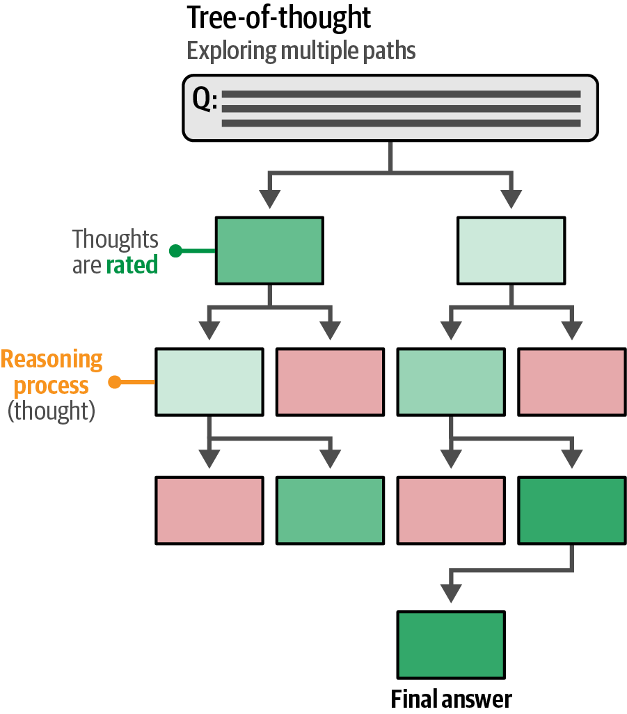
Tree-of-Thought excels at tasks requiring exploration of multiple paths, such as creative writing, but its reliance on numerous generative model calls can be slow.
A more efficient approach involves prompting the model to simulate a multi-expert discussion to reach a consensus, mimicking the ToT framework with a single call.
# zero-shot tree-of-thought prompt
zeroshot_tot_prompt = [
    {
        'role': 'user',
        'content': "Imagine three different experts are answering this question. All experts will write down 1 step of their thinking, then share it with the group. Then all experts will go on to the next step, etc. If any expert realizes they're wrong at any point then they leave. The question is 'The cafeteria had 23 apples. If they used 20 to make lunch and bought 6 more, how many apples do they have?' Make sure to discuss the results.",
    }
]

# generate the output
outputs = pipe(zeroshot_tot_prompt)
print(outputs[0]['generated_text'])
**Expert 1:**
Step 1: Start with the initial number of apples, which is 23.
**Expert 2:**
Step 1: Subtract the apples used for lunch, which is 20, from the initial 23 apples. This leaves 3 apples.
**Expert 3:**
Step 1: Add the 6 apples that were bought to the remaining 3 apples. This results in 9 apples.
**Discussion:**
All three experts agree on the final result. The cafeteria started with 23 apples, used 20 for lunch, leaving them with 3 apples. Then, they bought 6 more apples, bringing the total to 9 apples. Therefore, the cafeteria now has 9 apples.6.6. Output Verification
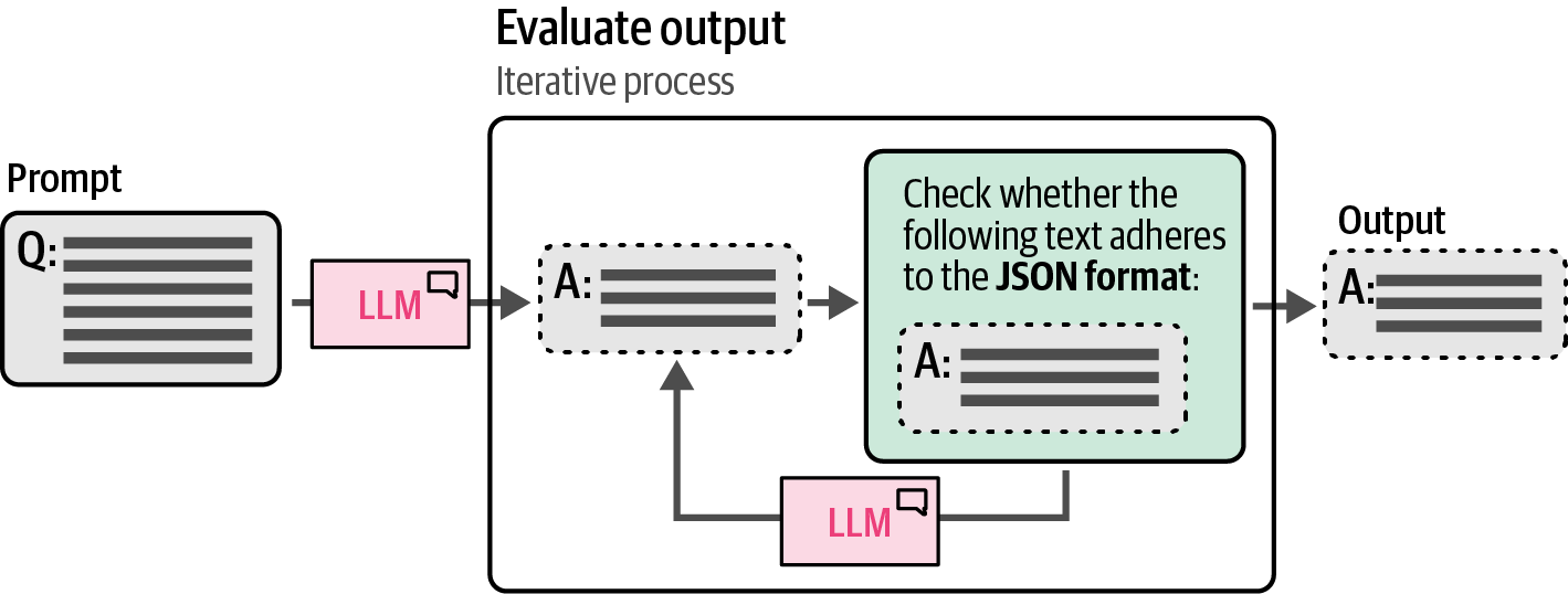
Systems and applications built with generative models might eventually end up in production. When that happens, it is important to verify and control the output of the model to prevent breaking the application and to create a robust generative AI application.
-
By default, most generative models create free-form text without adhering to specific structures other than those defined by natural language.
Some use cases require their output to be structured in certain formats, like JSON.
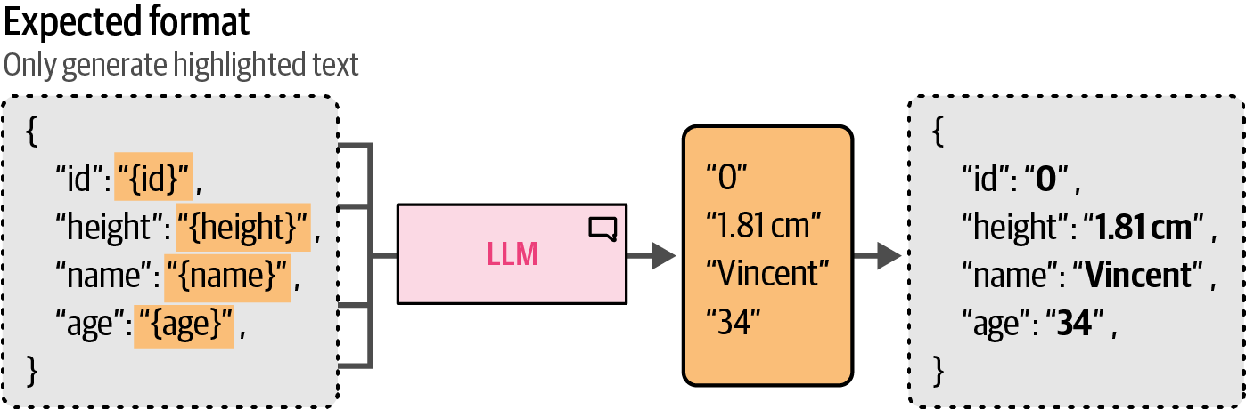
-
Even allowing the model to generate structured output, it still has the capability to freely generate its content.
For instance, when a model is asked to output either one of two choices, it should not come up with a third.
-
Some open source generative models have no guardrails and will generate outputs that do not consider safety or ethical considerations.
For instance, use cases might require the output to be free of profanity, personally identifiable information (PII), bias, cultural stereotypes, etc.
-
Many use cases require the output to adhere to certain standards or performance.
The aim is to double-check whether the generated information is factually accurate, coherent, or free from hallucination.
Generally, there are three ways of controlling the output of a generative model:
-
Examples: Provide a number of examples of the expected output.
-
Grammar: Control the token selection process.
-
Fine-tuning: Tune a model on data that contains the expected output.
6.6.1. Providing Examples
A simple and straightforward method to fix the output is to provide the generative model with examples of what the output should look like.
The few-shot learning is a helpful technique that guides the output of the generative model, which can be generalized to guide the structure of the output as well.
| An important note here is that it is still up to the model whether it will adhere to your suggested format or not. Some models are better than others at following instructions. |
# zero-shot learning: providing no in-context examples
zeroshot_prompt = [
    {
        'role': 'user',
        'content': 'Create a character profile for an RPG game in JSON format.',
    }
]

# generate the output
outputs = pipe(zeroshot_prompt)
print(outputs[0]['generated_text'])

# one-shot learning: providing a single in-context example of the desired output structure
one_shot_template = '''Create a short character profile for an RPG game. Make
sure to only use this format:
{
  "description": "A SHORT DESCRIPTION",
  "name": "THE CHARACTER'S NAME",
  "armor": "ONE PIECE OF ARMOR",
  "weapon": "ONE OR MORE WEAPONS"
}
'''
one_shot_prompt = [{'role': 'user', 'content': one_shot_template}]

# generate the output
outputs = pipe(one_shot_prompt)
print(outputs[0]['generated_text'])
{
"name": "Eldrin Shadowbane",
"class": "Rogue",
"level": 10,
"race": "Elf",
"background": "Eldrin was born into a noble family in the elven city of Luminara. He was trained in the arts of stealth and combat from a young age. However, Eldrin always felt a deep connection to the shadows and the mysteries of the night. He left his family to become a rogue
{
"description": "A skilled archer with a mysterious past, known for their agility and precision.",
"name": "Lyra Swiftarrow",
"armor": "Leather bracers and a lightweight leather tunic",
"weapon": "Longbow, throwing knives"
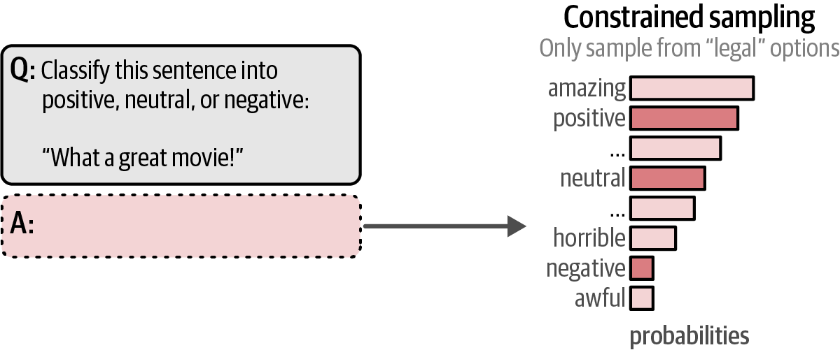
}6.6.2. Grammar: Constrained Sampling
Few-shot learning has a significant disadvantage: explicitly preventing certain output is not possible. Although the model is guided and given instructions, it might still not follow them completely.
Grammar-constrained sampling is a technique used during the token generation process of a Large Language Model (LLM) that enforces adherence to predefined grammars or rules when selecting the next token.
Instead, packages have been rapidly developed to constrain and validate the output of generative models, like Guidance, Guardrails, and LMQL, which leverage generative models to validate their own output.
Like transformers, llama-cpp-python is a library, generally used to efficiently load and use compressed models (quantization) in the GGUF format but can also be used to apply a JSON grammar.
from llama_cpp.llama import Llama

# load the Phi-3 language model using the llama-cpp-python library
llm = Llama.from_pretrained(
    repo_id="microsoft/Phi-3-mini-4k-instruct-gguf",
    filename="*fp16.gguf",
    n_gpu_layers=-1,
    n_ctx=2048,
    verbose=False,
)

# generate output using the loaded language model for a chat completion task
output = llm.create_chat_completion(
    messages=[
        {
            "role": "user",
            "content": "Create a warrior for an RPG in JSON for mat.",
        },
    ],
    response_format={"type": "json_object"}, # specify the response_format as a JSON
    temperature=0,
)['choices'][0]['message']["content"]

import json

# check whether the output actually is JSON
json_output = json.dumps(json.loads(output), indent=4)
print(json_output)
{
"warrior": {
"name": "Aldarion the Brave",
"class": "Warrior",
"level": 10,
"attributes": {
"strength": 18,
"dexterity": 10,
"constitution": 16,
"intelligence": 8,
"wisdom": 10,
"charisma": 12
},7. Advanced Text Generation Techniques and Tools
LangChain is a framework for developing applications powered by large language models (LLMs), which implements a standard interface for large language models and related technologies, such as embedding models and vector stores, and integrates with hundreds of providers.
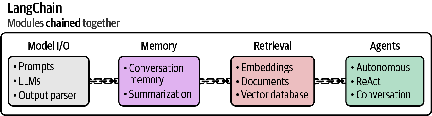
|
Hugging Face models can be run locally through the |
7.1. Model I/O: Loading Quantized Models with LangChain
A GGUF model represents a compressed version of its original counterpart through a method called quantization, which reduces the number of bits needed to represent the parameters of an LLM.
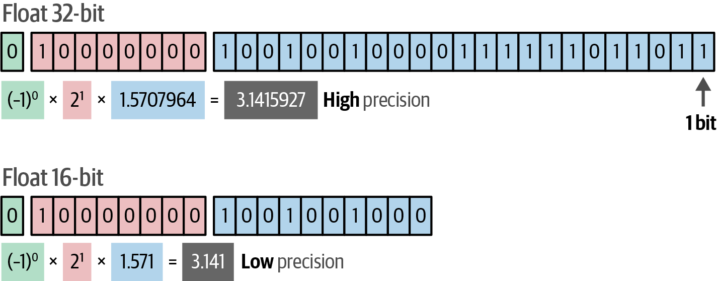
-
Bits, a series of 0s and 1s, represent values through binary encoding; more bits allow for a wider range of values but demand greater memory for storage.
-
Quantization reduces the number of bits required to represent the parameters of an LLM while attempting to maintain most of the original information.
Quantization comes with some loss in precision but often makes up for it as the model is much faster to run, requires less VRAM, and is often almost as accurate as the original.
Like rounding the time to the nearest minute ("14:16") instead of including seconds ("14:16 and 12 seconds"), quantization reduces the precision of a value without losing essential information.
As a rule of thumb, look for at least 4-bit quantized models. These models have a good balance between compression and accuracy. Although it is possible to use 3-bit or even 2-bit quantized mod‐ els, the performance degradation becomes noticeable and it would instead be preferable to choose a smaller model with a higher precision.
-
To download a specific bit-variant file (e.g., fp16) of the microsoft/Phi-3-mini-4k-instruct-gguf model, which includes multiple files with different bit-variants (see the 'Files and versions' tab).
# download from the primary Hugging Face URL: wget https://huggingface.co/microsoft/Phi-3-mini-4k-instruct-gguf/resolve/main/Phi-3-mini-4k-instruct-fp16.gguf # alternatively, download from the HF mirror: wget https://hf-mirror.com/microsoft/Phi-3-mini-4k-instruct-gguf/resolve/main/Phi-3-mini-4k-instruct-fp16.gguf -
Use Llama.cpp together with LangChain to load the GGUF file, and generate output.
# !wget https://huggingface.co/microsoft/Phi-3-mini-4k-instruct-gguf/resolve/main/Phi-3-mini-4k-instruct-fp16.gguf
# !pip install llama-cpp-python langchain_communit
from langchain_community.llms import LlamaCpp

# initialize the LlamaCpp language model integration from Langchain
llm = LlamaCpp(
    # path to the downloaded GGUF model file (ensure this file exists!)
    model_path="Phi-3-mini-4k-instruct-fp16.gguf",
    n_gpu_layers=-1,
    max_tokens=500,
    n_ctx=2048,
    seed=42,
    verbose=False,
)

# invoke the language model with a prompt.
output = llm.invoke("Hi! My name is Maarten. What is 1 + 1?")

# no/meanless output! Phi-3 requires a specific prompt template.
print(output)
7.2. Chains: Extending the Capabilities of LLMs
In Langchain, a "chain" is a core concept that goes beyond running LLMs in isolation, which involves connecting an LLM with other components like prompts, tools, or even other chains, to enhance its capabilities and create more complex systems.
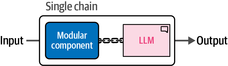
7.2.1. A Single Link in the Chain: Prompt Template
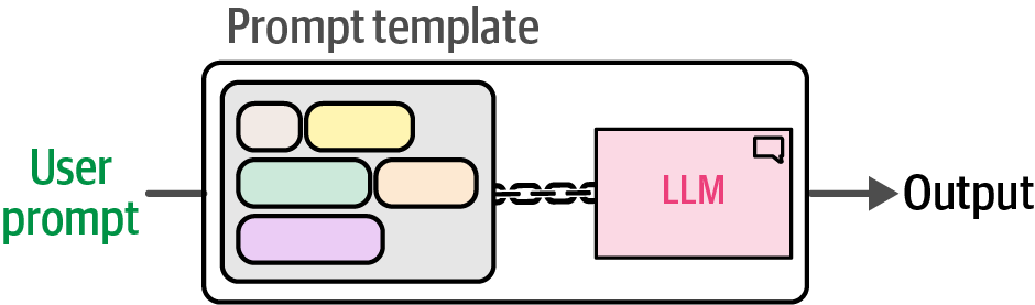
By chaining a prompt template with an LLM to get the output, only the user and system prompts need to be defined for each interaction, eliminating the need to repeatedly define the full prompt template.
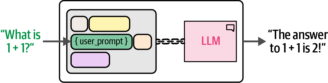
The template for Phi-3 is comprised of four main components:
-
<s>to indicate when the prompt starts -
<|user|>to indicate the start of the user’s prompt -
<|assistant|>to indicate the start of the model’s output -
<|end|>to indicate the end of either the prompt or the model’s output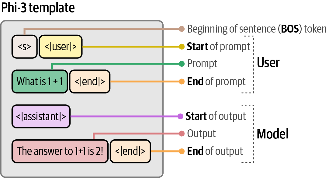 Figure 82. The prompt template Phi-3 expects.
from langchain_core.prompts import PromptTemplate

# create a prompt template with a placeholder for the user's input
template = """<s><|user|> {input_prompt}<|end|> <|assistant|>"""
prompt = PromptTemplate(
    template=template,
    input_variables=["input_prompt"],
)

# create a simple chain with the prompt template and the language model
basic_chain = prompt | llm

# invoke the chain with the input for the prompt template
output = basic_chain.invoke(
    {
        "input_prompt": "Hi! My name is Maarten. What is 1 + 1?",
    }
)

# the 'output' variable now contains the generated text
print(output)
Hello Maarten! The answer to 1 + 1 is 2.7.2.2. A Chain with Multiple Prompts
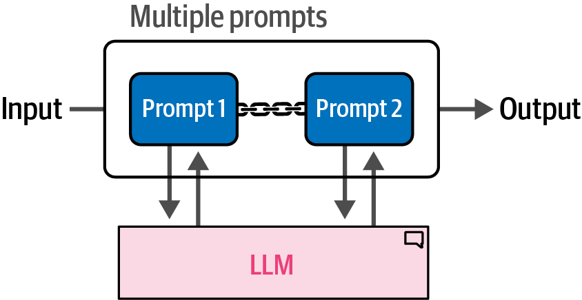
A multiple prompt chain, or sequential chain, processes a complex task by dividing it into a series of smaller, sequential subtasks, where each subtask utilizes a distinct prompt and LLM call, with the output from one step feeding directly into the input of the subsequent step.
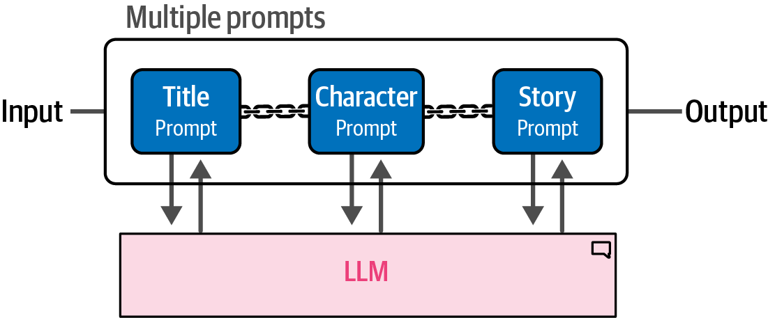
import json
from langchain_core.prompts import PromptTemplate
from langchain_core.runnables import RunnablePassthrough, RunnableLambda
from langchain.schema import StrOutputParser
from langchain_openai import ChatOpenAI

llm = ChatOpenAI(
    model='qwen2.5:0.5b-instruct',
    temperature=0.7,
    max_tokens=100,
    timeout=30,
    max_retries=2,
    base_url='http://localhost:11434/v1', # Ollama API
    api_key='API-KEY',
    verbose=True,
)

title_prompt = PromptTemplate.from_template(
    "<s><|user|>"
    "Create a title for a story about {summary}."
    "Only return the title."
    "<|end|> <|assistant|>"
)
character_prompt = PromptTemplate.from_template(
    "<s><|user|>"
    "Describe the main character of a story about {summary} with the title {title}. "
    "Use only two sentences."
    "<|end|><|assistant|>"
)
story_prompt = PromptTemplate.from_template(
    "<s><|user|>"
    "Create a story about {summary} with the title {title}."
    "The main character is: {character}. "
    "Only return the story and it cannot be longer than one paragraph."
    "<|end|><|assistant|>"
)

# LCEL-style chain using Runnables
title_chain = (
    {"summary": RunnablePassthrough()} | title_prompt | llm | StrOutputParser()
)

character_chain = (
    {"summary": RunnablePassthrough(), "title": title_chain}
    | character_prompt
    | llm
    | StrOutputParser()
)

story_chain = (
    {
        "summary": RunnablePassthrough(),
        "title": title_chain,
        "character": character_chain,
    }
    | story_prompt
    | llm
    | StrOutputParser()
)

aggregate_chain = RunnableLambda(
    lambda inputs: {
        "summary": inputs["summary"],
        "title": inputs["title"],
        "character": inputs["character"],
        "story": inputs["story"],
    }
)

final_chain = {
    "summary": RunnablePassthrough(),
    "title": title_chain,
    "character": character_chain,
    "story": story_chain,
} | aggregate_chain

output = final_chain.invoke({"summary": "a girl that lost her mother"})
print(json.dumps(output, indent=2))
{
"summary": {
"summary": "a girl that lost her mother"
},
"title": "\"Lost Mother Girl\"",
"character": "In the story, the main character named Lily, who was born to an ordinary family, unexpectedly finds herself the daughter of a rich individual after losing her mother. She navigates this new reality with courage and strength, learning valuable lessons about empathy, perseverance, and the power of resilience.",
"story": "In the quiet village where Linxue lived, her mother had been gone for many years. As an only child, she often felt distant from the other children in the village. One day,7.3. Memory: Helping LLMs to Remember Conversations
Memory can be added to the LLM chain using methods like conversation buffers and conversation summaries to make chat models stateful to remember previous conversations.
7.3.1. Conversation Buffer
In Langchain, ConversationBufferMemory provides an intuitive way to give LLMs memory by updating the prompt to include the full chat history.
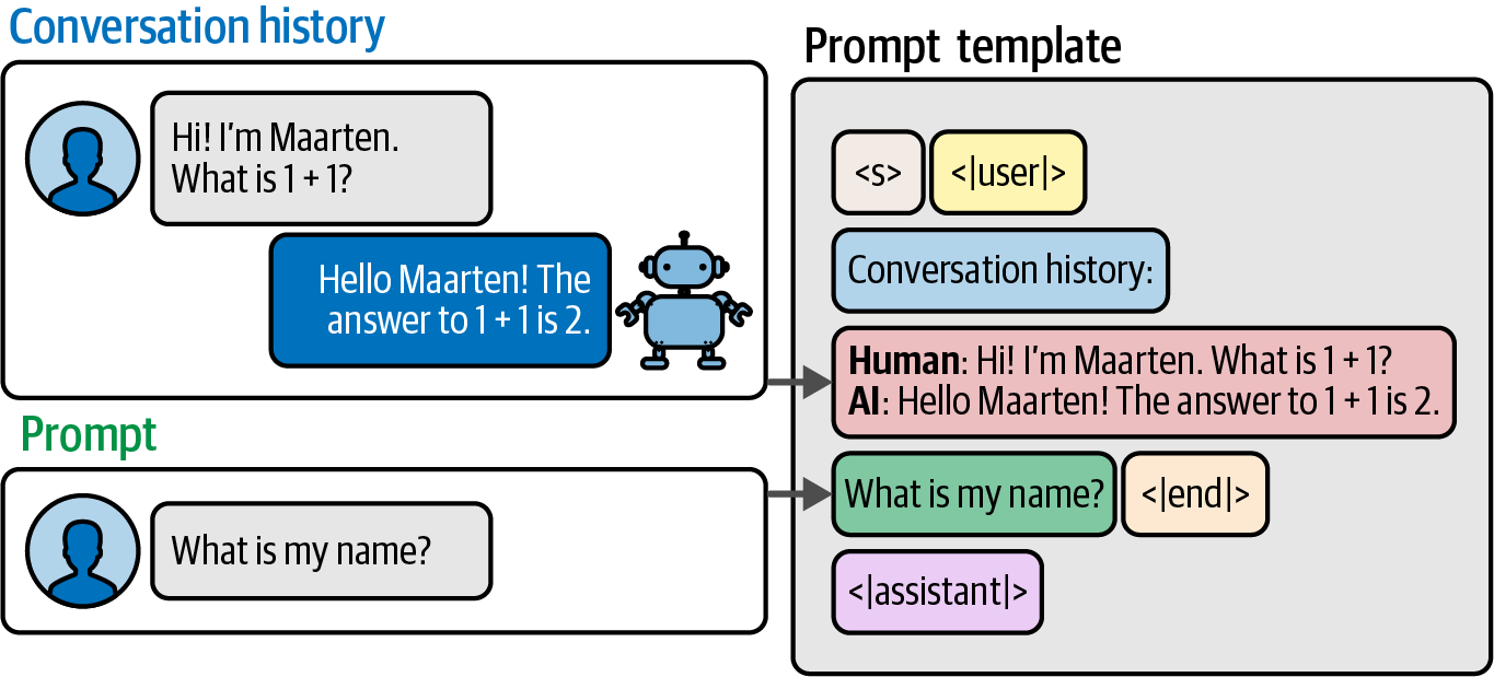
from langchain_core.prompts import PromptTemplate

template = """<s><|user|>Current conversation:{chat_history}

{input}<|end|>
<|assistant|>"""
prompt = PromptTemplate.from_template(template)

from langchain.memory import ConversationBufferMemory

memory = ConversationBufferMemory(memory_key="chat_history")

from langchain.chains.llm import LLMChain

llm_chain = LLMChain(prompt=prompt, llm=llm, memory=memory)llm_chain.invoke({"input": "Hi! My name is Maarten. What is 1 + 1?"}){'input': 'Hi! My name is Maarten. What is 1 + 1?',
'chat_history': '',
'text': 'Nice to meet you, Maarten!\n\nThe answer to 1 + 1 is... 2!'}llm_chain.invoke({"input": "What is my name?"}){'input': 'What is my name?',
'chat_history': 'Human: Hi! My name is Maarten. What is 1 + 1?\nAI: Nice to meet you, Maarten!\n\nThe answer to 1 + 1 is... 2!',
'text': 'Nice to meet you too, Maarten! Your name is indeed Maarten. Would you like to ask another question or have a conversation?'}7.3.2. Windowed Conversation Buffer
In LangChain, ConversationBufferWindowMemory decides how many the last k conversations are passed to the input prompt.
from langchain_core.prompts import PromptTemplate

template = """<s><|user|>Current conversation:{chat_history}

{input}<|end|>
<|assistant|>"""
prompt = PromptTemplate.from_template(template)

from langchain.memory import ConversationBufferWindowMemory

memory = ConversationBufferWindowMemory(k=2, memory_key="chat_history")

from langchain.chains.llm import LLMChain

llm_chain = LLMChain(prompt=prompt, llm=llm, memory=memory)

llm_chain.invoke(
    input="Hi! My name is Maarten and I am 33 years old. What is 1 + 1?"
)
llm_chain.invoke(input="What is 3 + 3?")
llm_chain.invoke({"input": "What is my name?"})
llm_chain.invoke({"input": "What is my age?"})
7.3.3. Conversation Summary
In LangChain, ConversationSummaryMemory summarizes the entire conversation history (typically using an external LLM) before providing it to the input prompt.
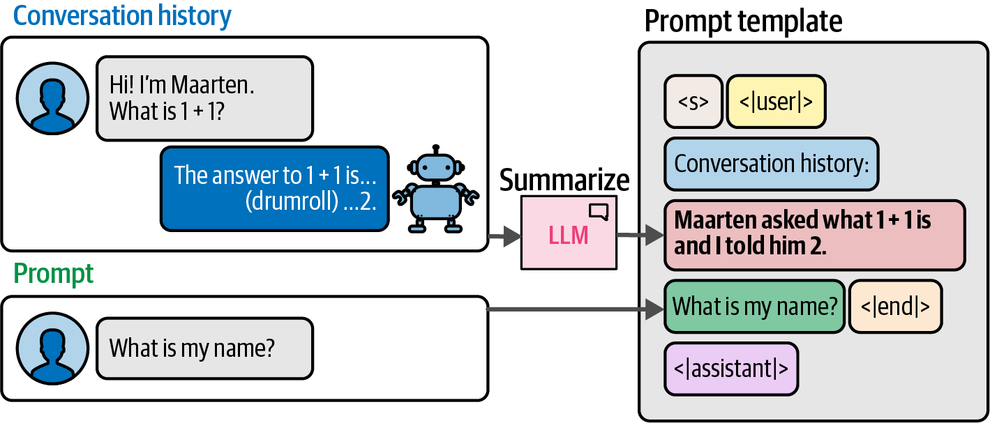
from langchain_core.prompts import PromptTemplate

template = """<s><|user|>Current conversation:{chat_history}

{input}<|end|>
<|assistant|>"""
prompt = PromptTemplate.from_template(template)

from langchain.memory import ConversationSummaryMemory

# prepare a summarization template as the summarization prompt
summary_prompt_template = """<s><|user|>Summarize the conversations and update
with the new lines.
Current summary:
{summary}
new lines of conversation:
{new_lines}
New summary:<|end|>
<|assistant|>"""
summary_prompt = PromptTemplate.from_template(template=summary_prompt_template)

memory = ConversationSummaryMemory(
    llm=llm, memory_key="chat_history", prompt=summary_prompt
)

from langchain.chains.llm import LLMChain

llm_chain = LLMChain(prompt=prompt, llm=llm, memory=memory)llm_chain.invoke({"input": "Hi! My name is Maarten. What is 1 + 1?"}){'input': 'Hi! My name is Maarten. What is 1 + 1?',
'chat_history': '',
'text': 'Hi Maarten!\n\nThe answer to 1 + 1 is 2.'}llm_chain.invoke({"input": "What is my name?"}){'input': 'What is my name?',
'chat_history': "Here is the updated summary:\n\nCurrent summary:\n\n* Human: Hi! My name is Maarten. What is 1 + 1?\n* AI: Hi Maarten!\n* Answer: The answer to 1 + 1 is 2.\n\nNew lines of conversation:\nHuman: That's correct, what's 2 * 2?\nAI: Let me calculate... The answer to 2 * 2 is 4.",
'text': 'Hi Maarten! Your name was mentioned earlier in our conversation. You said "Hi! My name is Maarten." What can I help you with next?'}llm_chain.invoke({"input": "What was the first question I asked?"}){'input': 'What was the first question I asked?',
'chat_history': 'Here\'s the updated summary:\n\nCurrent summary:\n\n* Human: Hi! My name is Maarten. What is 1 + 1?\n* AI: Hi Maarten!\n* Answer: The answer to 1 + 1 is 2.\n* Human: That\'s correct, what\'s 2 * 2?\n* AI: Let me calculate... The answer to 2 * 2 is 4.\n* Human: What is my name?\n* AI: Hi Maarten! Your name was mentioned earlier in our conversation. You said "Hi! My name is Maarten." What can I help you with next?',
'text': 'The first question you asked was: "what\'s 1 + 1?"'}# check what the summary is thus far
memory.load_memory_variables({}){'chat_history': 'Here is the updated summary:\n\nCurrent summary:\n\n* Human: Hi! My name is Maarten. What is 1 + 1?\n* AI: Hi Maarten!\n* Answer: The answer to 1 + 1 is 2.\n* Human: That\'s correct, what\'s 2 * 2?\n* AI: Let me calculate... The answer to 2 * 2 is 4.\n* Human: What is my name?\n* AI: Hi Maarten! Your name was mentioned earlier in our conversation. You said "Hi! My name is Maarten." What can I help you with next?\n* Human: What was the first question I asked?\n* AI: The first question you asked was: "what\'s 1 + 1?"'}7.4. Agents: Creating a System of LLMs
Agents are systems that take a high-level task and use an LLM as a reasoning engine to decide what actions to take and execute those actions.
ReAct (Reasoning and Acting) is a cognitive framework for language models that interleaves reasoning ("Thoughts") and acting ("Actions") with observations, allowing the model to dynamically plan, execute, and learn from its interactions with external tools or environments to solve complex tasks.
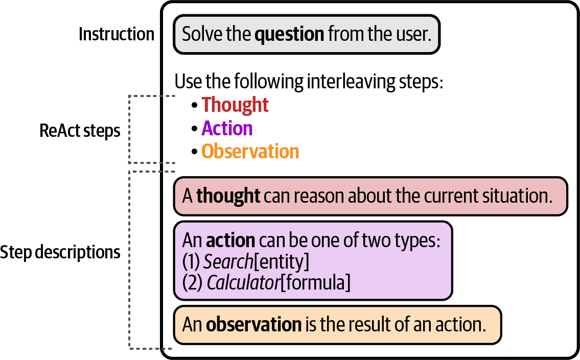
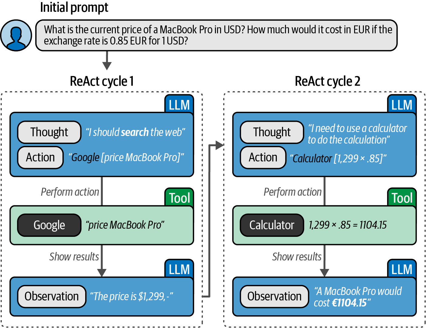
from langchain_openai import ChatOpenAI

# an LLM that is powerful enough to properly follow complex instructions
llm = ChatOpenAI(
    model="mistral:7b-instruct", # "llama3.1:8b", # "llama3.2:1b",
    temperature=0.7,
    max_tokens=100,
    base_url="http://localhost:11434/v1",
    api_key="API-KEY",
    verbose=True,
)

from langchain_core.prompts import PromptTemplate

# create the ReAct template
react_template = """Answer the following questions as best you can. You have
access to the following tools:

{tools}

Use the following format:

Question: the input question you must answer
Thought: you should always think about what to do
Agents: Creating a System of LLMs
Action: the action to take, should be one of [{tool_names}]
Action Input: the input to the action
Observation: the result of the action
... (this Thought/Action/Action Input/Observation can repeat N times)
Thought: I now know the final answer
Final Answer: the final answer to the original input question

Begin!

Question: {input}
Thought:{agent_scratchpad}"""

prompt = PromptTemplate(
    template=react_template,
    input_variables=["tools", "tool_names", "input", "agent_scratchpad"],
)

from langchain.agents import load_tools, Tool
from langchain_community.tools.ddg_search.tool import DuckDuckGoSearchResults

search = DuckDuckGoSearchResults()
search_tool = Tool(
    name="duckduck",
    description="A web search engine. Use this to as a search engine for general queries.",
    func=search.run,
)

tools = load_tools(["llm-math"], llm=llm)
tools.append(search_tool)

from langchain.agents import AgentExecutor, create_react_agent

agent = create_react_agent(llm, tools, prompt)
agent_executor = AgentExecutor(
    agent=agent,
    tools=tools,
    verbose=True,
    handle_parsing_errors=True,
    max_iterations=5,
)agent_executor.invoke(
{
"input": "What is 123 + 456?"
}
)> Entering new AgentExecutor chain...
To solve this, I will use the Calculator tool. The input for the calculator will be the equation "123 + 456".
Action: Calculator
Action Input: "123 + 456"Answer: 579 I now know the final answer.
Final Answer: The result of the calculation (123 + 456) is 579.
> Finished chain.
{'input': 'What is 123 + 456?',
'output': 'The result of the calculation (123 + 456) is 579.'}agent_executor.invoke(
{
"input": "What is the current price of a MacBook Pro in USD? How much would it cost in EUR if the exchange rate is 0.85 EUR for 1 USD."
}
)> Entering new AgentExecutor chain...
I need to find the current price of a MacBook Pro and then convert that price from USD to EUR using the given exchange rate.
Agents: Calculator, duckduck
Action: duckduck
Action Input: What is the current price of a MacBook Pro in USD?snippet: Apple resellers are hosting a variety of MacBook Pro sales that discount current M4, M4 Pro and M4 Max 14-inch and 16-inch models, in addition to blowout bargains on M3 models. Apple offers two ..., title: Best MacBook Pro Deals for March 2025 | Save up to $1,200 - AppleInsider, link: https://appleinsider.com/deals/best-macbook-pro-deals, snippet: The newly launched M4 Pro and M4 Max 14-inch MacBook Pros have shown notable performance improvements over their M1, M2, and M3 counterparts, especially in single-core scores. In recent benchmarks, the M4 Pro 14-inch MacBook Pro achieved a single-core score of approximately 3,850, surpassing the M3 Pro's single-core score by about 15-20%., title: Apple 14″ MacBook Pro Prices at MacPrices.net, link: https://www.macprices.net/14-macbook-pro/, snippet: Apple MacBook Pro 14" (M4/512GB): was $1,599 now $1,399 at Amazon. The M4-based MacBook Pro M4 is pretty close to being the perfect laptop. You get fantastic performance from the M4 chip, useful ..., title: Epic Apple MacBook sale is live — shop the best deals from $629 right ..., link: https://www.tomsguide.com/sales-events/epic-apple-macbook-sale-is-live-shop-the-best-deals-from-usd629-right-now, snippet: The M4 Max MacBook Pro is Apple's most powerful option, and both the silver and space black options are on sale. ... List price Best price (current) Best price (all-time) M2 MacBook Air (13-inch ..., title: Best MacBook Deals: Save on Apple's Latest Laptops and Previous-Gen ..., link: https://www.cnet.com/deals/best-macbook-deals/ The current price of a MacBook Pro in USD can be found from the search results. Let me filter the results a bit more specifically to find the price.
Agents: duckduck
Action: duckduck
Action Input: What is the price of a new 14-inch MacBook Pro (M4/512GB) in USD?snippet: - 14″ M4 MacBook Pro (16GB/1TB/Gray): $1599, $200 off MSRP - 14″ M4 MacBook Pro (24GB/1TB/Gray): $1799, $200 off MSRP. These are currently the lowest prices available for new M4-powered 14″ MacBook Pros among the Apple retailers we track. For the latest sales and prices, keep an eye on our 14-inch MacBook Pro Price Tracker, updated daily., title: 14-inch M4 MacBook Pros on sale today for $150-$200 off MSRP, link: https://www.macprices.net/2025/01/14/14-inch-m4-macbook-pros-on-sale-today-for-150-200-off-msrp/, snippet: Every M4 Pro and M4 Max model is also on sale at up to $300 off in our Mac Price Guide. Prices start at $1,699. Here are a few top picks from the MacBook Pro sale: 14-inch M4, 16GB, 512GB, Space ..., title: Apple M4 MacBook Pro Drops to $1,399, Free Next Day Shipping - AppleInsider, link: https://appleinsider.com/articles/24/12/25/snag-an-m4-macbook-pro-14-inch-for-1399-with-free-next-day-delivery, snippet: The M4 Pro MacBook Pro 14-inch has hit a new record low price of $1,699, with units in stock with free store pickup as early as today. But don't delay, as the deal ends on Christmas Eve., title: Apple MacBook Pro 14-inch M4 Pro Drops to Best $1,699 Price - AppleInsider, link: https://appleinsider.com/articles/24/12/24/apples-14-inch-macbook-pro-with-m4-pro-chip-plunges-to-record-low-1699-today-only, snippet: Right now the 14-inch MacBook Pro is available with a discount that slashes its price to the lowest yet, and you won't want to miss out. Amazon is now selling the M4 MacBook Pro for just $1,398 ..., title: Apple's Latest M4 14-inch MacBook Pro Is Now Yours for Its Best-Ever Price, link: https://www.cnet.com/deals/apples-latest-m4-14-inch-macbook-pro-is-now-yours-for-its-best-ever-price/ The current price of a new 14-inch MacBook Pro (M4/512GB) in USD is $1399. To find the cost in EUR, we can use the given exchange rate of 0.85 EUR for 1 USD. So, the cost of the MacBook Pro in EUR would be 1399 * 0.85 = €1176.21.
Final Answer: The current price of a new 14-inch MacBook Pro (M4/512GB) is approximately €1176.21 in EUR.
> Finished chain.
{'input': 'What is the current price of a MacBook Pro in USD? How much would it cost in EUR if the exchange rate is 0.85 EUR for 1 USD.',
'output': 'The current price of a new 14-inch MacBook Pro (M4/512GB) is approximately €1176.21 in EUR.'}Appendix A: LangChain
LangChain is a framework that consists of a number of packages, which implements a standard interface for large language models and related technologies, such as embedding models and vector stores, and integrates with hundreds of providers.

-
langchain-coreis a lightweight package containing base abstractions and interfaces for core Langchain components like chat models, vector stores, and tools, without including any third-party integrations and with minimal dependencies. -
langchainis the main package containing generic chains and retrieval strategies that form an application’s cognitive architecture, independent of specific third-party integrations. -
Integrations are a list of lightweight packages (e.g.,
langchain-openai,langchain-anthropic) that contain specific integrations and are co-maintained for proper versioning. -
langchain-communityis a package containing third-party integrations for various components (chat models, vector stores, tools, etc.), maintained by the Langchain community, with all dependencies being optional to ensure a lightweight package. -
langgraphis an extension oflangchainaimed at building robust and stateful multi-actor applications with LLMs by modeling steps as edges and nodes in a graph. -
langserveis a package to deploy LangChain chains as REST APIs that makes it easy to get a production ready API up and running. -
LangSmith is a developer platform for debugging, testing, evaluating, and monitoring LLM applications.
7.A.1. Chat Models and Messages
Large Language Models (LLMs) are advanced machine learning models that excel in a wide range of language-related tasks such as text generation, translation, summarization, question answering, and more, without needing task-specific fine tuning for every scenario.
LangChain provides a consistent interface for working with chat models from different providers that takes a list of messages as input and returns a message as output while offering additional features for monitoring, debugging, and optimizing the performance of applications that use LLMs.
LangChain supports two message formats to interact with chat models:
-
LangChain Message Format: LangChain’s own message format, which is used by default and is used internally by LangChain.
-
OpenAI’s Message Format: OpenAI’s message format.
Messages are the unit of communication in chat models, which are used to represent the input and output of a chat model, as well as any additional context or metadata that may be associated with a conversation.
-
Each message has a role (e.g., "user", "assistant") and content (e.g., text, multimodal data) with additional metadata that varies depending on the chat model provider.
-
LangChain provides a unified message format that can be used across chat models, allowing users to work with different chat models without worrying about the specific details of the message format used by each model provider.
-
LangChain messages are Python objects that subclass from a
BaseMessage.-
SystemMessage: corresponds tosystemrole -
HumanMessage: corresponds touserrole -
AIMessage: corresponds toassistantrole -
AIMessageChunk: corresponds toassistantrole, used for streaming responses -
ToolMessage: corresponds totoolrole
-
|
When invoking a chat model with a string as input, LangChain will automatically convert the string into a |
from langchain_openai import ChatOpenAI

llm = ChatOpenAI(
    model="gpt-4o",
    temperature=0,
    max_tokens=100,
    timeout=30,
    max_retries=2,
)

llm.invoke('What is LangChain?')
7.A.2. Prompt Templates
Prompt Templates are responsible for formatting user input into a format that can be passed to a language model, take as input a dictionary, where each key represents a variable in the prompt template to fill in, and output a PromptValue.
from langchain_core.prompts import PromptTemplate

prompt_template = PromptTemplate.from_template("Tell me a joke about {topic}")
prompt = prompt_template.format(**{"topic": "cats"})
print(prompt)
# Tell me a joke about cats
from langchain_core.prompts import ChatPromptTemplate
prompt_template = ChatPromptTemplate([
("system", "You are a helpful assistant"),
("user", "Tell me a joke about {topic}")
])
prompt = prompt_template.format(**{"topic": "cats"})
print(prompt)
# System: You are a helpful assistant
# Human: Tell me a joke about catsfrom langchain_core.prompts import ChatPromptTemplate, MessagesPlaceholder
from langchain_core.messages import HumanMessage
prompt_template = ChatPromptTemplate([
("system", "You are a helpful assistant"),
MessagesPlaceholder("msgs")
])
prompt = prompt_template.format(**{"msgs": [HumanMessage(content="hi!")]})
print(prompt)
# System: You are a helpful assistant
# Human: hi!
# alternatively
prompt_template = ChatPromptTemplate([
("system", "You are a helpful assistant"),
("placeholder", "{msgs}") # <-- This is the changed part
])
prompt = prompt_template.format(**{"msgs": [HumanMessage(content="hi!")]})
print(prompt)
# System: You are a helpful assistant
# Human: hi!7.A.3. Structured Outputs
Structured outputs are a concept where language models are instructed to respond in a structured format, rather than in direct natural language, which is useful in scenarios where the output needs to be machine-readable, such as storing output in a database and ensure that the output conforms to the database schema.
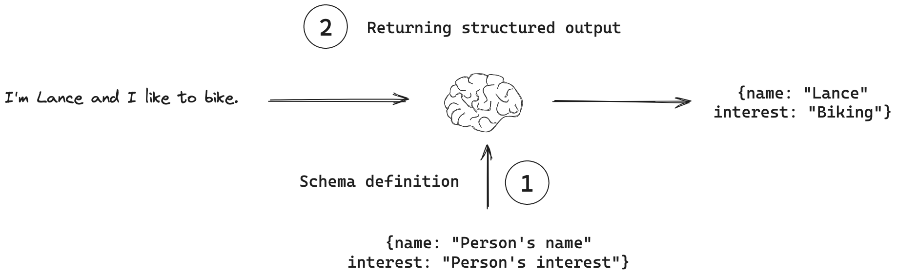
-
LangChain provides a method,
with_structured_output(), that automates the process of binding the schema to the model and parsing the output.from pydantic import BaseModel, Field class ResponseFormatter(BaseModel): """Always use this tool to structure your response to the user.""" answer: str = Field(description="The answer to the user's question") followup_question: str = Field(description="A followup question the user could ask") llm_with_structure = llm.with_structured_output(ResponseFormatter) structured_output = llm_with_structure.invoke( "What is the powerhouse of the cell?", verbose=True ) structured_outputResponseFormatter(answer='The powerhouse of the cell is the mitochondria.', followup_question='What is the organelle that powers the cell?') -
While one approach is to include defined schema in the prompt and ask nicely for the model to use it, it is not recommended.
from langchain.output_parsers.structured import ResponseSchema, StructuredOutputParser response_schemas = [ ResponseSchema( name="answer", description="The answer to the user's question", type="string", ), ResponseSchema( name="followup_question", description="A followup question the user could ask", type="string", ), ] parser = StructuredOutputParser.from_response_schemas(response_schemas) format_instructions = parser.get_format_instructions() from langchain.prompts import PromptTemplate prompt = PromptTemplate( template="{query}\n{format_instructions}\n", input_variables=["query"], partial_variables={"format_instructions": format_instructions}, )print(prompt.format(**{"query": "What is the powerhouse of the cell?"}))What is the powerhouse of the cell? The output should be a markdown code snippet formatted in the following schema, including the leading and trailing "```json" and "```": ```json { "answer": string // The answer to the user's question "followup_question": string // A followup question the user could ask } ```chain = prompt | llm | parser output = chain.invoke({"query": "What is the powerhouse of the cell?"}) output{'answer': 'The powerhouse of the cell is the nucleus.', 'followup_question': 'What does the nucleus play a crucial role in?'}
7.A.4. Output Parsers
Output Parsers are responsible for taking the output of a model and transforming it to a more suitable format for downstream tasks, which are useful when using LLMs to generate structured data, or to normalize output from chat models and LLMs.
# parse text from message objects
from langchain_core.output_parsers import StrOutputParser

chain = llm | StrOutputParser()

output = chain.invoke('What is 2 + 2 ?')
print(output)

# 2 + 2 equals 4.
# use output parsers to parse an LLM response into structured format
from langchain_core.output_parsers import PydanticOutputParser
from langchain_core.prompts import PromptTemplate
from pydantic import BaseModel, Field, model_validator
class Joke(BaseModel):
setup: str = Field(description="question to set up a joke")
punchline: str = Field(description="answer to resolve the joke")
parser = PydanticOutputParser(pydantic_object=Joke)
prompt = PromptTemplate(
template="Answer the user query.\n{format_instructions}\n{query}\n",
input_variables=["query"],
partial_variables={"format_instructions": parser.get_format_instructions()},
)
chain = prompt | llm | parser
output = chain.invoke({"query": "Tell me a joke."})
print(output.model_dump_json(indent=2))
# {
# "setup": "Why did the tomato turn red?",
# "punchline": "Because it saw the salad dressing!"
# }# parse JSON output
from langchain_core.output_parsers import JsonOutputParser
from langchain_core.prompts import PromptTemplate
from pydantic import BaseModel, Field
class Joke(BaseModel):
setup: str = Field(description="question to set up a joke")
punchline: str = Field(description="answer to resolve the joke")
parser = JsonOutputParser(pydantic_object=Joke)
instructions = parser.get_format_instructions()
print(f'\n{instructions}\n---------------')
prompt = PromptTemplate(
template="Answer the user query.\n{format_instructions}\n{query}\n",
input_variables=["query"],
partial_variables={"format_instructions": parser.get_format_instructions()},
)
chain = prompt | llm | parser
output = chain.invoke({"query": "Tell me a joke."})
print(output)
# The output should be formatted as a JSON instance that conforms to the JSON schema below.
#
# As an example, for the schema {"properties": {"foo": {"title": "Foo", "description": "a list of strings", "type": "array", "items": {"type": "string"}}}, "required": ["foo"]}
# the object {"foo": ["bar", "baz"]} is a well-formatted instance of the schema. The object {"properties": {"foo": ["bar", "baz"]}} is not well-formatted.
#
# Here is the output schema:
# ```
# {"properties": {"setup": {"description": "question to set up a joke", "title": "Setup", "type": "string"}, "punchline": {"description": "answer to resolve the joke", "title": "Punchline", "type": "string"}}, "required": ["setup", "punchline"]}
# ```
# ---------------
# {'setup': 'Why did the tomato turn red?', 'punchline': 'Because it saw the salad dressing!'}7.A.5. Embedding, Vector Stores, and Retrievers
Embedding models are machine learning models that transform human language or multimodal data (text, audio, images, video - not currently fully supported by Langchain) into numerical vector representations (embeddings), which are fixed-length arrays capturing the semantic meaning of the input, enabling machines to understand and compare data based on conceptual similarity, not just keywords.
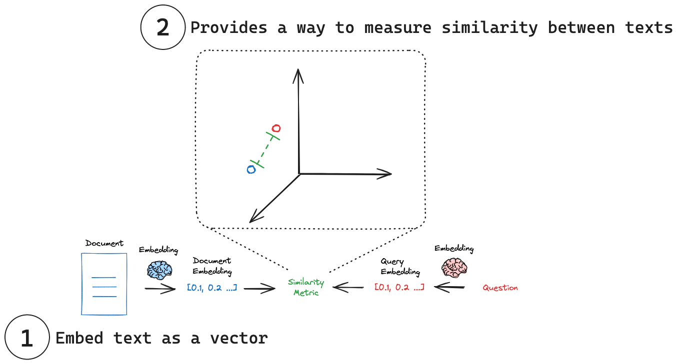
-
(1) Embed text as a vector: Embeddings transform text into a numerical vector representation.
-
(2) Measure similarity: Embedding vectors can be compared using simple mathematical operations.
LangChain provides a universal interface for working with embedding models, providing standard methods for common operations, and simplifies interaction with various embedding providers through two central methods:
-
embed_documents: For embedding multiple texts (documents) -
embed_query: For embedding a single text (query)# for embedding multiple texts (documents) from langchain_openai import OpenAIEmbeddings embeddings_model = OpenAIEmbeddings() embeddings = embeddings_model.embed_documents( [ "Hi there!", "Oh, hello!", "What's your name?", "My friends call me World", "Hello World!" ] ) len(embeddings), len(embeddings[0]) (5, 1536)# for embedding a single text (query) query_embedding = embeddings_model.embed_query("What is the meaning of life?")# measure similarity import numpy as np def cosine_similarity(vec1, vec2): dot_product = np.dot(vec1, vec2) norm_vec1 = np.linalg.norm(vec1) norm_vec2 = np.linalg.norm(vec2) return dot_product / (norm_vec1 * norm_vec2) similarity = cosine_similarity(query_result, document_result) print("Cosine Similarity:", similarity)# hugging face embeddings from langchain_huggingface import HuggingFaceEmbeddings embeddings = HuggingFaceEmbeddings(model_name="sentence-transformers/all-MiniLM-L6-v2") query_embedding = embeddings.embed_query("Hello, world!") print(len(query_embedding)) # 384
Vector stores are databases that can efficiently store and retrieve embeddings, which are frequently used to search over unstructured data, such as text, images, and audio, to retrieve relevant information based on semantic similarity rather than exact keyword matches.

LangChain provides a standard interface for working with vector stores, allowing users to easily switch between different vectorstore implementations. The key methods are:
-
add_documents: Add a list of texts to the vector store. -
delete: Delete a list of documents from the vector store. -
similarity_search: Search for similar documents to a given query.
from langchain_huggingface import HuggingFaceEmbeddings

embeddings = HuggingFaceEmbeddings(model_name="sentence-transformers/all-MiniLM-L6-v2")

from langchain_core.vectorstores import InMemoryVectorStore

# initialize with an embedding model
vector_store = InMemoryVectorStore(embedding=embeddings)

# add documents
from langchain_core.documents import Document

document_1 = Document(
    page_content="I had chocalate chip pancakes and scrambled eggs for breakfast this morning.",
    metadata={"source": "tweet"},
)

document_2 = Document(
    page_content="The weather forecast for tomorrow is cloudy and overcast, with a high of 62 degrees.",
    metadata={"source": "news"},
)

documents = [document_1, document_2]

vector_store.add_documents(documents=documents)
# ['df0f6926-c824-4114-a2c5-2b19d9d8740c', 'fa105761-9dd6-4c1c-860a-28e3e4ba181a']

# provide IDs for the documents to the vector store
vector_store.add_documents(documents=documents, ids=["doc1", "doc2"])
# ['doc1', 'doc2']

# delete documents
vector_store.delete(ids=["doc1"])

# similarity search
query = "my query"
docs = vectorstore.similarity_search(query)
print(docs[0].page_content)
Retrievers in Langchain are components that provide a unified way to interact with various retrieval systems, including vector stores, graph databases, and relational databases, and take a natural language query as input to return a list of relevant documents.
-
LangChain provides a uniform interface for interacting with different types of retrieval systems that accepts a query and return documents.
-
A Langchain retriever is a
runnable, which is a standard interface for Langchain components, and it has a few common methods, includinginvoke, that are used to interact with it.docs = retriever.invoke(query)
Lost in the Middle is the phenomenon where Large Language Models (LLMs) have difficulty effectively using information located in the middle of a long input context, often performing better when relevant details are at the beginning or end.
-
Documents retrieved from vector stores are typically returned in descending order of relevance, often measured by cosine similarity of embeddings.
-
To mitigate the "lost in the middle" effect, re-order documents after retrieval such that the most relevant documents are positioned at extrema (e.g., the first and last pieces of context), and the least relevant documents are positioned in the middle.
-
The
LongContextReorderdocument transformer implements the re-ordering procedure.from langchain_huggingface import HuggingFaceEmbeddings embeddings = HuggingFaceEmbeddings( model_name="sentence-transformers/all-MiniLM-L6-v2" ) from langchain_core.vectorstores import InMemoryVectorStore texts = [ "Basquetball is a great sport.", "Fly me to the moon is one of my favourite songs.", "The Celtics are my favourite team.", "This is a document about the Boston Celtics", "I simply love going to the movies", "The Boston Celtics won the game by 20 points", "This is just a random text.", "Elden Ring is one of the best games in the last 15 years.", "L. Kornet is one of the best Celtics players.", "Larry Bird was an iconic NBA player.", ] vector_store = InMemoryVectorStore.from_texts(texts, embedding=embeddings) from langchain_core.runnables import chain from langchain_core.documents import Document # create a retriever @chain def retriever(query: str) -> list[Document]: docs, scores = zip(*vector_store.similarity_search_with_score(query, k=10)) for doc, score in zip(docs, scores): doc.metadata["score"] = score return docs docs = retriever.invoke(query) max_score_length = max(len(f"{doc.metadata['score']:.6f}") for doc in docs) for doc in docs: score_str = f"{doc.metadata['score']:.6f}".rjust(max_score_length) print(f"- {score_str}: {doc.page_content}")- 0.675469: This is a document about the Boston Celtics - 0.638917: The Celtics are my favourite team. - 0.552694: L. Kornet is one of the best Celtics players. - 0.460651: The Boston Celtics won the game by 20 points - 0.320224: Larry Bird was an iconic NBA player. - 0.244521: Elden Ring is one of the best games in the last 15 years. - 0.231564: Basquetball is a great sport. - 0.106447: I simply love going to the movies - 0.059917: Fly me to the moon is one of my favourite songs. - 0.034081: This is just a random text.from langchain_community.document_transformers import LongContextReorder # Reorder the documents: # Less relevant document will be at the middle of the list and more # relevant elements at beginning / end. reordering = LongContextReorder() reordered_docs = reordering.transform_documents(docs) # Confirm that the 4 relevant documents are at beginning and end. for doc in reordered_docs: score_str = f"{doc.metadata['score']:.6f}".rjust(max_score_length) print(f"- {score_str}: {doc.page_content}")- 0.638917: The Celtics are my favourite team. - 0.460651: The Boston Celtics won the game by 20 points - 0.244521: Elden Ring is one of the best games in the last 15 years. - 0.106447: I simply love going to the movies - 0.034081: This is just a random text. - 0.059917: Fly me to the moon is one of my favourite songs. - 0.231564: Basquetball is a great sport. - 0.320224: Larry Bird was an iconic NBA player. - 0.552694: L. Kornet is one of the best Celtics players. - 0.675469: This is a document about the Boston Celtics
7.A.6. Document Loaders
Document Loaders are responsible for loading documents from a variety of sources.
# simple and fast text extraction

from langchain_community.document_loaders import PyPDFLoader

file_path = "./books/llm-book.pdf"

loader = PyPDFLoader(file_path)
pages = []
for page in loader.lazy_load():
    pages.append(page)

print(f"{pages[0].metadata}\n")
print(pages[0].page_content)
{'source': './books/llm-book.pdf', 'page': 0, 'page_label': 'Cover'}
Hands-On
Large Language
Models
Language Understanding
and Generation
Jay Alammar &
Maarten Grootendorst# vector search over PDFs
from langchain_core.vectorstores import InMemoryVectorStore
from langchain_huggingface import HuggingFaceEmbeddings
embeddings = HuggingFaceEmbeddings(
model_name="sentence-transformers/all-MiniLM-L6-v2"
)
vector_store = InMemoryVectorStore.from_documents(pages, embeddings)
docs = vector_store.similarity_search("What is Prompt Engineering?", k=2)
for doc in docs:
print(f'Page {doc.metadata["page"]}: {doc.page_content[:300]}\n')Page 194: Intro to Prompt Engineering
An essential part of working with text-generative LLMs is prompt engineering. By
carefully designing our prompts we can guide the LLM to generate desired responses.
Whether the prompts are questions, statements, or instructions, the main goal of
prompt engineering is to e
Page 219: Summary
In this chapter, we explored the basics of using generative models through prompt
engineering and output verification. We focused on the creativity and potential com‐
plexity that comes with prompt engineering. These components of a prompt are key
in generating and optimizing output appropri7.A.7. Text Splitters
Text splitters split documents into smaller, manageable chunks for use in downstream applications, particularly retrieval systems, to handle non-uniform document lengths, overcome model limitations, improve representation quality, enhance retrieval precision, and optimize computational resources.
Text splitting approaches include length-based methods (token or character), text-structure based methods (like recursive splitting that respects paragraphs and sentences), document-structure based methods (leveraging formats like Markdown or HTML), and semantic meaning based methods (analyzing content for significant meaning shifts).
from langchain_text_splitters import RecursiveCharacterTextSplitter

text_splitter = RecursiveCharacterTextSplitter(
    chunk_size=100,
    chunk_overlap=20,
    length_function=len,
    is_separator_regex=False,
)
with open("state_of_the_union.txt") as f:
state_of_the_union = f.read()
texts = text_splitter.split_text(state_of_the_union)
print(texts[0])
print(texts[1])Madam Speaker, Madam Vice President, our First Lady and Second Gentleman. Members of Congress and
of Congress and the Cabinet. Justices of the Supreme Court. My fellow Americans.from langchain_community.document_loaders.text import TextLoader
loader = TextLoader("state_of_the_union.txt")
documents = loader.load()
split_documents = text_splitter.split_documents(documents)
print(split_documents[0])
print(split_documents[1])page_content='Madam Speaker, Madam Vice President, our First Lady and Second Gentleman. Members of Congress and' metadata={'source': 'state_of_the_union.txt'}
page_content='of Congress and the Cabinet. Justices of the Supreme Court. My fellow Americans.' metadata={'source': 'state_of_the_union.txt'}from langchain_community.document_loaders import PyPDFLoader
loader = PyPDFLoader("./books/llm-book.pdf")
documents = loader.load()
split_documents = text_splitter.split_documents(documents)
print(split_documents[0])
print(split_documents[1])page_content='Hands-On
Large Language
Models
Language Understanding
and Generation
Jay Alammar &' metadata={'source': './books/llm-book.pdf', 'page': 0, 'page_label': 'Cover'}
page_content='Jay Alammar &
Maarten Grootendorst' metadata={'source': './books/llm-book.pdf', 'page': 0, 'page_label': 'Cover'}7.A.8. Tools
LangChain’s tool abstraction links a Python function to a schema defining its name, description, and expected arguments, which chat models that support tool calling (or function calling) can use to request the execution of a specific function with specific inputs
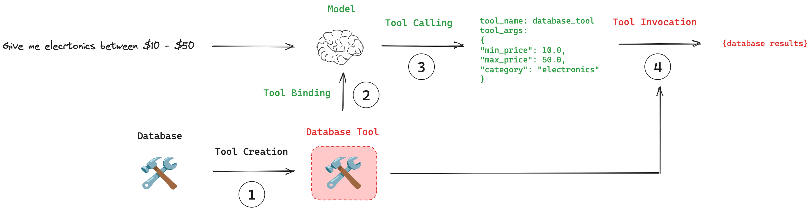
-
A key principle of tool calling is that the model decides when to use a tool based on the input’s relevance.
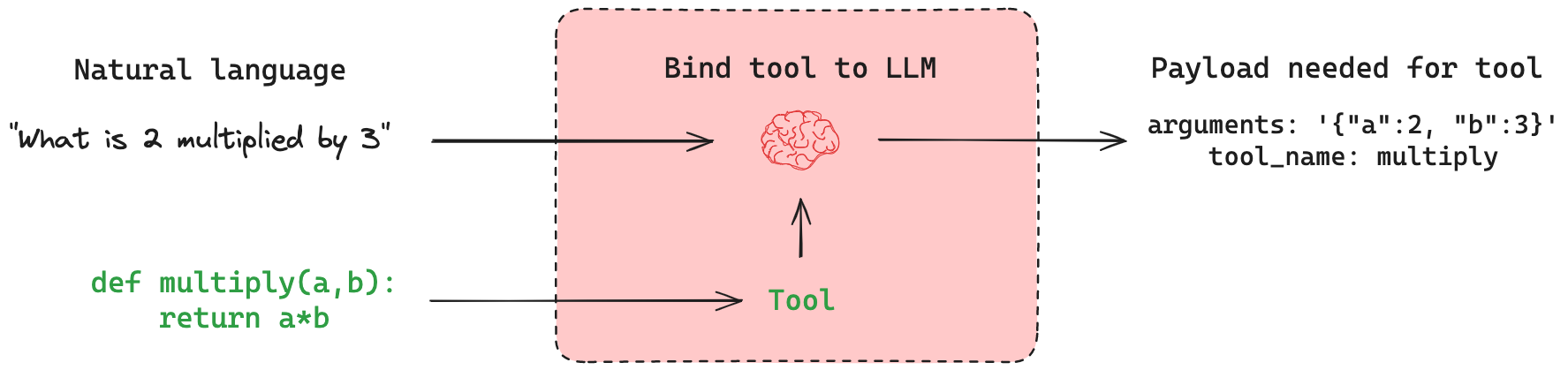
# tool creation
@tool
def multiply(a: int, b: int) -> int:
    """Multiply a and b."""
    return a * b

tools = [multiply]

# tool binding
llm_with_tools = llm.bind_tools(tools)
# tool calling output = llm_with_tools.invoke("What is 2 multiplied by 3?") output.content, output.tool_calls('', [{'name': 'multiply', 'args': {'a': 2, 'b': 3}, 'id': 'call_zerallda', 'type': 'tool_call'}])# model doesn't always need to call a tool output = llm_with_tools.invoke("Hello world!") output.content, output.tool_calls('Hello! How can I assist you today?', [])
7.A.9. Chat History
Chat history is sequence of messages, each of which is associated with a specific role, such as user, assistant, system, or tool, a record of the conversation between the user and the chat model, which is used to maintain context and state throughout the conversation.
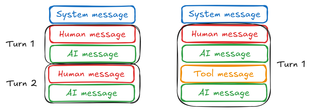
A full conversation often starts with a system message that sets the context for the conversation, and follows a combination of two alternating message patterns: user and assistant, representing a back-and-forth conversation, or assistant and tool, representing an "agentic" workflow where the assistant invokes tools for specific tasks.
All models have finite context windows, and trim_messages can be used to reduce the size of a chat history to a specified token count or specified message count.
from langchain_core.messages import (
    AIMessage,
    HumanMessage,
    SystemMessage,
    trim_messages,
)

messages = [
    SystemMessage("you're a good assistant, you always respond with a joke."),
    HumanMessage("i wonder why it's called langchain"),
    AIMessage(
        'Well, I guess they thought "WordRope" and "SentenceString" just didn\'t have the same ring to it!'
    ),
    HumanMessage("and who is harrison chasing anyways"),
    AIMessage(
        "Hmmm let me think.\n\nWhy, he's probably chasing after the last cup of coffee in the office!"
    ),
    HumanMessage("what do you call a speechless parrot"),
]
# trimming based on token count
from langchain_core.messages.utils import count_tokens_approximately
trim_messages(
messages,
strategy="last",
token_counter=count_tokens_approximately,
max_tokens=45,
start_on="human",
end_on=("human", "tool"),
include_system=True,
allow_partial=False,
)SystemMessage(content="you're a good assistant, you always respond with a joke.", additional_kwargs={}, response_metadata={}),
HumanMessage(content='what do you call a speechless parrot', additional_kwargs={}, response_metadata={})]# trimming based on message count
trim_messages(
messages,
strategy="last",
token_counter=len,
max_tokens=5, # message count
start_on="human",
end_on=("human", "tool"),
include_system=True,
)[SystemMessage(content="you're a good assistant, you always respond with a joke.", additional_kwargs={}, response_metadata={}),
HumanMessage(content='and who is harrison chasing anyways', additional_kwargs={}, response_metadata={}),
AIMessage(content="Hmmm let me think.\n\nWhy, he's probably chasing after the last cup of coffee in the office!", additional_kwargs={}, response_metadata={}),
HumanMessage(content='what do you call a speechless parrot', additional_kwargs={}, response_metadata={})]# using a chat model as a token counter
from langchain_openai import ChatOpenAI
trim_messages(
messages,
max_tokens=45,
strategy="first",
token_counter=ChatOpenAI(model="gpt-4o"),
)# chaining
from langchain_openai import ChatOpenAI
llm = ChatOpenAI(model="gpt-4o")
trimmer = trim_messages(
token_counter=llm,
strategy="last",
max_tokens=45,
start_on="human",
end_on=("human", "tool"),
include_system=True,
)
chain = trimmer | llm
chain.invoke(messages)from langchain_core.chat_history import InMemoryChatMessageHistory
from langchain_core.runnables.history import RunnableWithMessageHistory
chat_history = InMemoryChatMessageHistory(messages=messages[:-1])
def dummy_get_session_history(session_id):
if session_id != "1":
return InMemoryChatMessageHistory()
return chat_history
trimmer = trim_messages(
max_tokens=45,
strategy="last",
token_counter=llm,
include_system=True,
start_on="human",
)
chain = trimmer | llm
chain_with_history = RunnableWithMessageHistory(
chain, dummy_get_session_history
)
chain_with_history.invoke(
[HumanMessage("what do you call a speechless parrot")],
config={"configurable": {"session_id": "1"}},
)7.A.10. Memory
Memory is a cognitive function that allows people to store, retrieve, and use information to understand their present and future. Short-term memory, or thread-scoped memory, can be recalled at any time from within a single conversational thread with a user. Long-term memory is shared across conversational threads, and can be recalled at any time and in any thread.
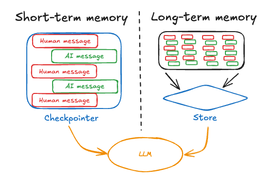
7.A.11. LangChain Expression Language (LCEL)
The LangChain Expression Language (LCEL) uses a declarative approach, similar to a Unix pipe, to build new Runnable components from existing ones, where a Runnable created with LCEL is often referred to as a "chain" and fully implements the Runnable interface.
from langchain_core.vectorstores import InMemoryVectorStore
from langchain_huggingface import HuggingFaceEmbeddings

embeddings = HuggingFaceEmbeddings(
    model_name="sentence-transformers/all-MiniLM-L6-v2"
)
vectorstore = InMemoryVectorStore.from_texts(
    ["harrison worked at kensho"],
    embedding=embeddings,
)
retriever = vectorstore.as_retriever()
from langchain_core.prompts import ChatPromptTemplate
template = """Answer the question based only on the following context:
{context}
Question: {question}
"""
prompt = ChatPromptTemplate.from_template(template)from langchain_core.runnables import RunnablePassthrough
prompt_chain = {
"context": retriever,
"question": RunnablePassthrough(),
} | prompt
prompt_text = prompt_chain.invoke("where did harrison work?").to_string()
print(prompt_text)Human: Answer the question based only on the following context:
[Document(id='d03a67c7-a031-43aa-a27c-6411f9dd0dba', metadata={}, page_content='harrison worked at kensho')]
Question: where did harrison work?from langchain_core.output_parsers import StrOutputParser
from langchain_openai import ChatOpenAI
llm = ChatOpenAI()
retrieval_chain = (
{"context": retriever, "question": RunnablePassthrough()}
| prompt
| llm
| StrOutputParser()
)
output = retrieval_chain.invoke("where did harrison work?")
print(output)Harrison worked at Kensho.In LCEL chains, the two main composition primitives are RunnableSequence and RunnableParallel.
-
RunnableSequenceis a composition primitive to chain multiple runnables sequentially, with the output of one runnable serving as the input to the next.from langchain_core.runnables import RunnableSequence chain = RunnableSequence([runnable1, runnable2]) final_output = chain.invoke(some_input)corresponds to the following:
output1 = runnable1.invoke(some_input) final_output = runnable2.invoke(output1) -
RunnableParallelis a composition primitive to run multiple runnables concurrently, with the same input provided to each.from langchain_core.runnables import RunnableParallel chain = RunnableParallel({ "key1": runnable1, "key2": runnable2, }) final_output = chain.invoke(some_input){ "key1": runnable1.invoke(some_input), "key2": runnable2.invoke(some_input), } -
The
|(pipe) operator have been overloaded to create aRunnableSequencefrom twoRunnables.chain = runnable1 | runnable2is Equivalent to:
chain = RunnableSequence([runnable1, runnable2])is Equivalent to:
chain = runnable1.pipe(runnable2) -
LCEL applies automatic type coercion to make it easier to compose chains.
-
Inside an LCEL expression, a dictionary is automatically converted to a
RunnableParallel.mapping = { "key1": runnable1, "key2": runnable2, } chain = mapping | runnable3is automatically converted to the following:
chain = RunnableSequence([RunnableParallel(mapping), runnable3]) -
Inside an LCEL expression, a function is automatically converted to a
RunnableLambda.def some_func(x): return x chain = some_func | runnable1is automatically converted to the following:
chain = RunnableSequence([RunnableLambda(some_func), runnable1])
-
-
A
dictobject defines data routing in LCEL by mapping keys to Runnables, functions, or static values, whileRunnablePassthroughduplicates data across the pipeline as a data conduit to orchestrate chain flow.chain = ( {"input": RunnablePassthrough()} # capture initial input | { "output": llm_chain, # generate LLM output "input": RunnablePassthrough() # maintain original input } ) # output: {"output": "LLM's answer", "input": "user's question"}
8. Semantic Search and Retrieval-Augmented Generation
Dense retrieval, reranking, and Retrieval-Augmented Generation (RAG) represent three significant strategies for enhancing search using language models.
-
Dense retrieval systems rely on the concept of embeddings, and turn the search problem into retrieving the nearest neighbors of the search query (after both the query and the documents are converted into embeddings).
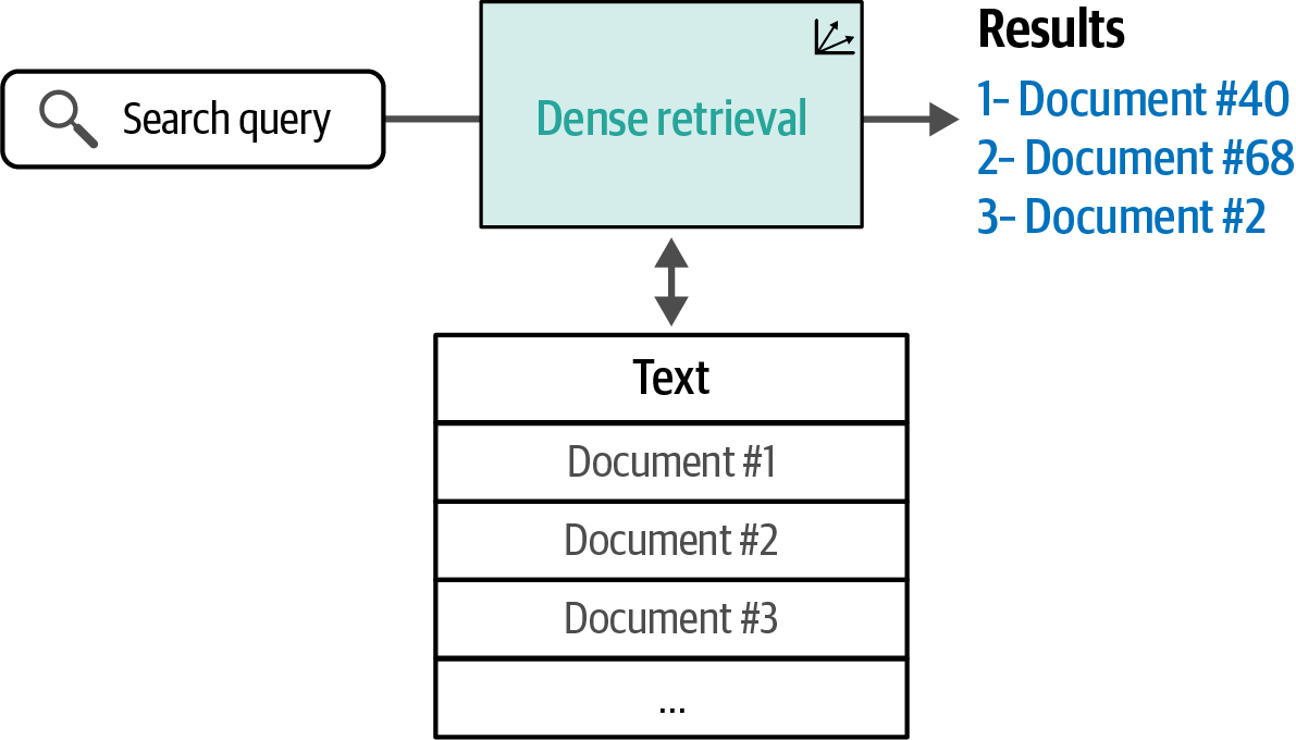 Figure 89. Dense retrieval is one of the key types of semantic search, relying on the similarity of text embeddings to retrieve relevant results.
 -
A reranking language model is one of multiple steps in search system pipelines and is tasked with scoring the relevance of a subset of results against the query; the order of results is then changed based on these scores.
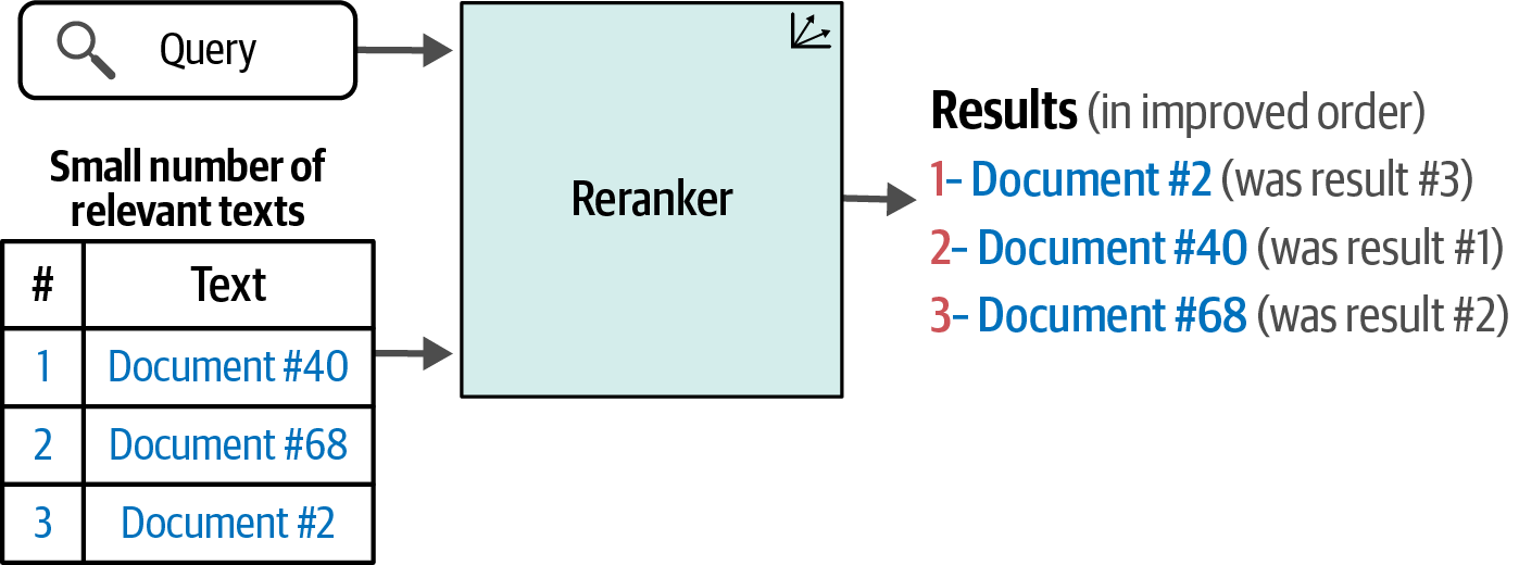 Figure 90. Rerankers, the second key type of semantic search, take a search query and a collection of results, and reorder them by relevance, often resulting in vastly improved results.
 -
An RAG (Retrieval-Augmented Generation) system is a text generation system that incorporates search capabilities to reduce hallucinations, increase factuality, and/or ground the generation model on a specific dataset.
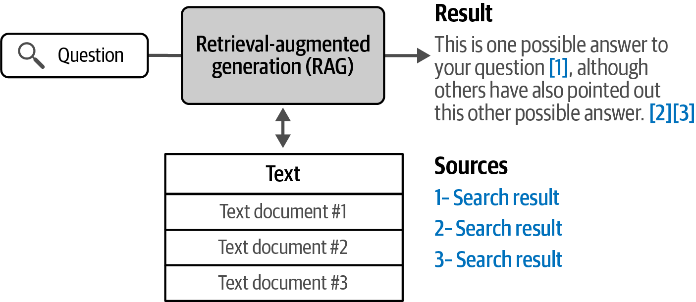 Figure 91. A RAG system formulates an answer to a question and (preferably) cites its information sources.
8.1. Semantic Search with Language Models
An embedding is a numeric representation of text, where each text is intuitively represented as a point (or a vector), and texts with similar meaning are close to each other in the high multi-dimensional embedding space.
8.1.1. Dense Retrieval
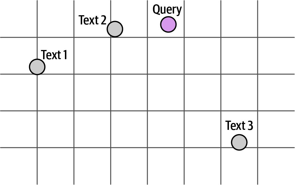
# dense retrieval with FAISS
from sentence_transformers import SentenceTransformer
import faiss

text = """
Artificial intelligence was founded as an academic discipline in 1956.
Alan Turing was the first person to conduct substantial research in AI.
Born in Maida Vale, London, Turing was raised in southern England.
"""
sentences = text.split(".")
sentences = [s.strip() for s in sentences if s.strip()]

model = SentenceTransformer("sentence-transformers/all-MiniLM-L6-v2")

# embedding the text chunks.
xb = model.encode(sentences)

# building the search index.
d = xb.shape[1]
index = faiss.IndexFlatL2(d)
index.add(xb)

# search the index
q = "Who is Alan Turing?"
xq = model.encode([q])
distances, indices = index.search(xq, 3)
print(f"Q: {q}")
for i in range(len(indices[0])):
    sentence = sentences[indices[0][i]]
    distance = distances[0][i]
    print(f"  Sentence: {sentence}")
    print(f"  Distance: {distance:.4f}")
Q: Who is Alan Turing?
Sentence: Alan Turing was the first person to conduct substantial research in AI
Distance: 0.4903
Sentence: Born in Maida Vale, London, Turing was raised in southern England
Distance: 1.0674
Sentence: Artificial intelligence was founded as an academic discipline in 1956
Distance: 1.4276# keyword search with BM25
import string
import numpy as np
from rank_bm25 import BM25Okapi
from sklearn.feature_extraction import _stop_words
from tqdm import tqdm
def bm25_tokenizer(text: str):
tokenized_doc = []
for token in text.lower().split():
token = token.strip(string.punctuation)
if len(token) > 0 and token not in _stop_words.ENGLISH_STOP_WORDS:
tokenized_doc.append(token)
return tokenized_doc
tokenized_corpus = []
text = """
Artificial intelligence was founded as an academic discipline in 1956.
Alan Turing was the first person to conduct substantial research in AI.
Born in Maida Vale, London, Turing was raised in southern England.
"""
texts = text.split('.')
for passage in tqdm(texts):
tokenized_corpus.append(bm25_tokenizer(passage))
bm25 = BM25Okapi(tokenized_corpus)
def keyword_search(q: str, k=3, n=3):
print("Input question:", q)
bm25_scores = bm25.get_scores(bm25_tokenizer(q))
top_n = np.argpartition(bm25_scores, -n)[-n:]
bm25_hits = [
{'corpus_id': idx, 'score': bm25_scores[idx]} for idx in top_n
]
bm25_hits = sorted(bm25_hits, key=lambda x: x['score'], reverse=True)
print("Top-3 lexical search (BM25) hits")
for hit in bm25_hits[0:k]:
print(
"\t{:.3f}\t{}".format(
hit['score'], texts[hit['corpus_id']].replace("\n", " ")
)
)
q = "Who is Alan Turing?"
keyword_search(q=q, k=3, n=len(texts))Input question: Who is Alan Turing?
Top-3 lexical search (BM25) hits
0.737 Alan Turing was the first person to conduct substantial research in AI
0.000 Artificial intelligence was founded as an academic discipline in 1956
0.000 Born in Maida Vale, London, Turing was raised in southern EnglandIt’s useful to be aware of some of the drawbacks of dense retrieval and how to address them.
-
Lack of Answer in Retrieved Texts
Dense retrieval always returns results based on semantic similarity, even if none of the texts actually contain the answer to the query. A potential solution is to implement a distance threshold to filter out results that are not sufficiently relevant. User feedback (click-through rates and satisfaction) can also help improve the system over time.
-
Difficulty with Exact Phrase Matches
Dense retrieval, relying on semantic similarity, may not perform well when a user is looking for an exact match of a specific phrase. In such cases, traditional keyword matching is more effective, suggesting the use of hybrid search systems that combine both approaches.
-
Domain Specificity
Dense retrieval models trained on data from one domain (e.g., internet and Wikipedia) may not generalize well to other, unseen domains (e.g., legal texts) without sufficient training data from that new domain.
-
Handling Multi-Sentence Answers
Dense retrieval systems face the challenge of how to best chunk long texts into embeddings. A key design parameter is deciding the optimal way to divide documents, as answers to some questions may span multiple sentences, and models have context size limitations. Chunking strategies include embedding per document (which can lose information) or embedding multiple chunks per document (which offers better coverage). Various chunking methods exist, such as by sentence, paragraph, or overlapping segments to retain context, with the best approach depending on the text and query types.
-
Scalability and Efficiency
While simple nearest neighbor search with tools like NumPy works for smaller datasets, for millions of vectors, optimized approximate nearest neighbor (ANN) search libraries like FAISS or Annoy are necessary for efficient retrieval. Vector databases like Weaviate or Pinecone offer additional functionalities like adding/deleting vectors without rebuilding the index and advanced filtering options.
-
Need for Fine-Tuning
To optimize dense retrieval for specific tasks, fine-tuning the embedding models with relevant query-result pairs (including negative examples) is crucial. This process aims to bring embeddings of relevant queries and results closer together in the vector space while pushing irrelevant ones further apart.
8.1.2. Reranking
A reranker takes in the search query and a number of search results, and returns the optimal ordering of these documents so the most relevant ones to the query are higher in ranking.
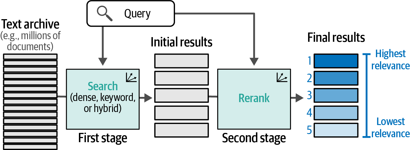
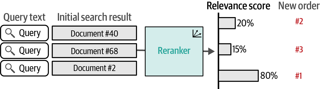
For the retrieval, either lexical search, e.g. with a vector engine like Elasticsearch, or dense retrieval with a SentenceTransformer (a.k.a. bi-encoder) can be used. However, the retrieval system might retrieve documents that are not that relevant for the search query. Hence, in a second stage, a re-ranker based on a CrossEncoder that scores the relevancy of all shortlisted candidates for the given search query can be used to output a ranked list.
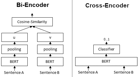
from sentence_transformers import SentenceTransformer

bi_encoder = SentenceTransformer("all-MiniLM-L6-v2")

corpus = [
    "A man is eating food.",
    "A man is eating a piece of bread.",
    "The girl is carrying a baby.",
    "A man is riding a horse.",
    "A woman is playing violin.",
    "Two men pushed carts through the woods.",
    "A man is riding a white horse on an enclosed ground.",
    "A monkey is playing drums.",
    "A cheetah is running behind its prey.",
]

corpus_embeddings = bi_encoder.encode(corpus, convert_to_tensor=True)

query = "A man is eating pasta."
query_embedding = bi_encoder.encode(query, convert_to_tensor=True)
top_N = min(10, len(corpus))
similarity_scores = bi_encoder.similarity(query_embedding, corpus_embeddings)[0]
import torch
scores, indices = torch.topk(similarity_scores, k=top_N)
documents = []
for score, index in zip(scores, indices):
document = corpus[index]
print(f"({score:.4f})", document)
documents.append(document)(0.7035) A man is eating food.
(0.5272) A man is eating a piece of bread.
(0.1889) A man is riding a horse.
(0.1047) A man is riding a white horse on an enclosed ground.
(0.0980) A cheetah is running behind its prey.
(0.0819) A monkey is playing drums.
(0.0336) A woman is playing violin.
(-0.0594) Two men pushed carts through the woods.
(-0.0898) The girl is carrying a baby.from sentence_transformers import CrossEncoder
cross_encoder = CrossEncoder("cross-encoder/ms-marco-MiniLM-L-6-v2")
top_K = min(5, top_N)
ranking = cross_encoder.rank(
query,
documents,
top_k=top_K,
return_documents=True,
)
for r in ranking:
print(f"({r['score']:.4f})", r["text"])(1.9005) A man is eating food.
(1.4804) A man is eating a piece of bread.
(-7.0890) A man is riding a horse.
(-8.9042) A man is riding a white horse on an enclosed ground.
(-10.7628) A monkey is playing drums.8.2. Retrieval-Augmented Generation (RAG)
RAG systems incorporate search capabilities in addition to generation capabilities to enhance factuality and reduce hallucinations.
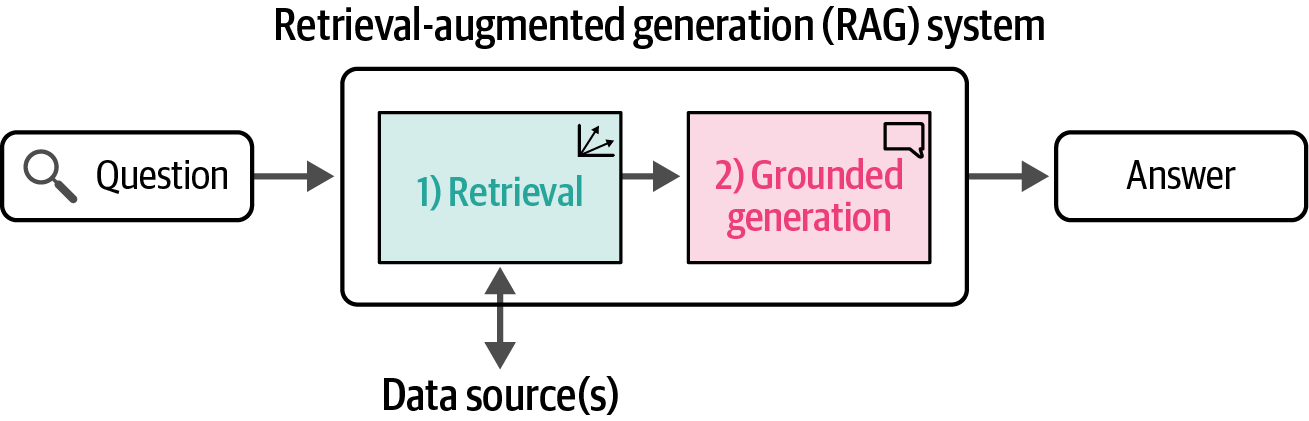
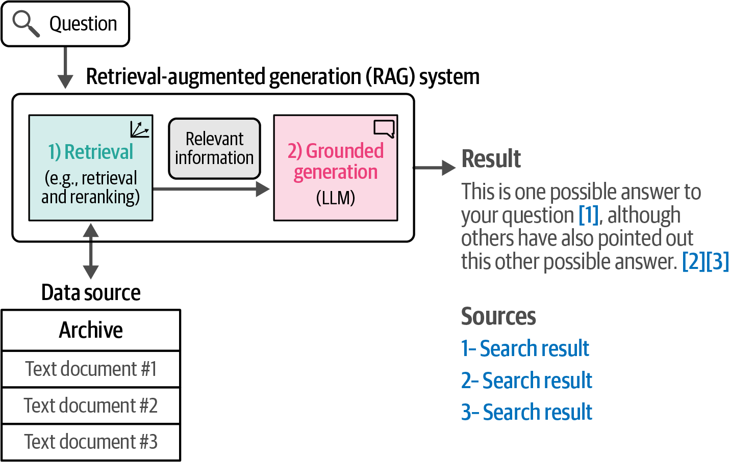
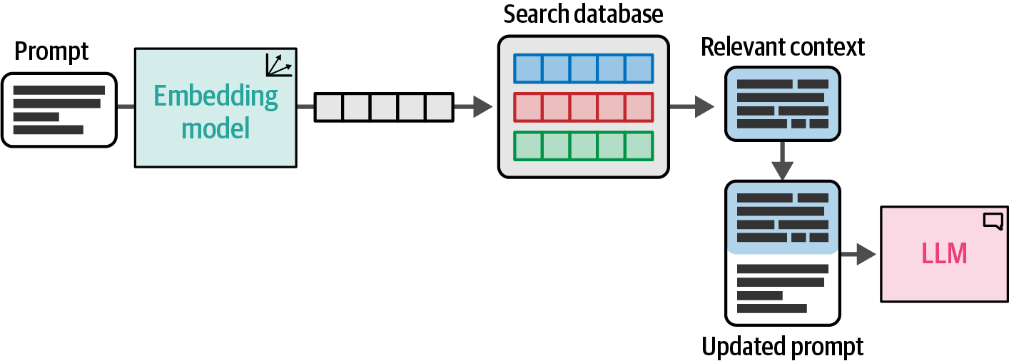
from langchain_openai import ChatOpenAI

llm = ChatOpenAI(
    model="mistral:7b-instruct",
    api_key='APK-KEY',
    base_url="http://localhost:11434/v1",  # Ollama
)
from langchain_text_splitters import HTMLHeaderTextSplitter
headers_to_split_on = [
("h1", "Header 1"),
("h2", "Header 2"),
("h3", "Header 3"),
("h4", "Header 4"),
]
html_splitter = HTMLHeaderTextSplitter(headers_to_split_on)
url = "https://plato.stanford.edu/entries/goedel/"
documents = html_splitter.split_text_from_url(url)from langchain_community.vectorstores import FAISS
from langchain_huggingface import HuggingFaceEmbeddings
embeddings = HuggingFaceEmbeddings(
model_name="sentence-transformers/all-MiniLM-L6-v2"
)
db = FAISS.from_documents(documents, embeddings)from langchain_core.prompts import PromptTemplate
template = """
Relevant information:
{context}
Provide a concise answer the following question using the relevant information
provided above:
{question}
"""
prompt = PromptTemplate.from_template(template=template)
from langchain.chains.retrieval_qa.base import RetrievalQA
rag = RetrievalQA.from_chain_type(
llm=llm,
chain_type="stuff",
retriever=db.as_retriever(),
chain_type_kwargs={"prompt": prompt},
verbose=True,
)rag.invoke("Who is Kurt Gödel?"){'query': 'Who is Kurt Gödel?',
'result': " Kurt Gödel was an Austrian mathematician and logician. He is best known for his work on the incompleteness theorems, which were established in 1930 and prove that any sufficiently rich formal axiomatic system contains either statements that cannot be proven or disproven within the system itself. Some of Gödel's other notable contributions include his proof of the consistency of the continuum hypothesis using large cardinals, and his work on undecidable propositions in number theory, which led to the concept of Gödel numbers for representing mathematical statements in a formal system. Throughout his life, Gödel also explored philosophical questions related to logic, mathematics, and metaphysics, including questions about realism, the foundations of mathematics, set theory, and the nature of time and truth."}9. Multimodal Large Language Models
A multimodal model is a type of artificial intelligence model capable of processing and reasoning across different modalities, where a modality refers to a distinct type of data such as text, images, audio, video, or sensor data.
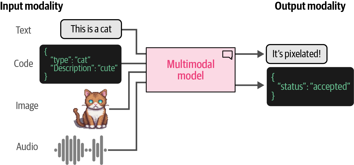
9.1. Vision Transformer (ViT)
Vision Transformer (ViT) is a method that adapts the Transformer architecture to the field of computer vision, particularly for image recognition tasks, by treating an image as a sequence of flattened image patches which are then linearly embedded and processed by the Transformer encoder in a manner similar to textual tokens, allowing it to capture global relationships in the image more directly than the local receptive fields of convolutional neural networks (CNNs).
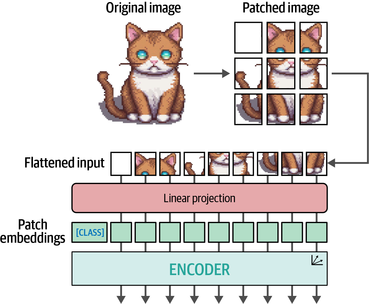
9.2. Multimodal Embedding Models
A multimodal embedding model is a type of model that can create numerical representations (embeddings) for multiple modalities, such as text and imagery, within the same vector space, allowing for direct comparison of representations from different modalities based on their semantic content.
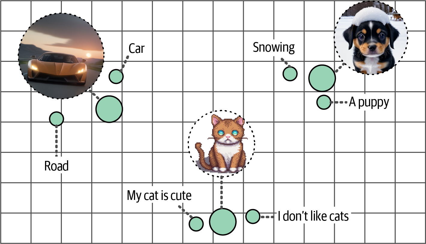
Contrastive Language-Image Pre-training (CLIP) is an embedding model to compute embeddings of both images and texts.
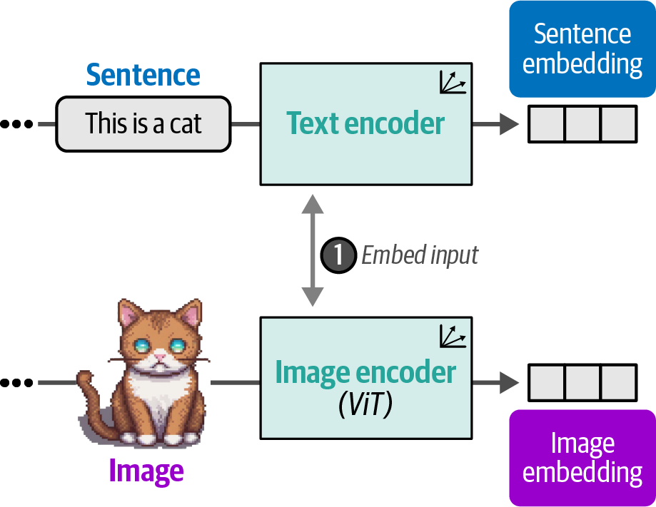
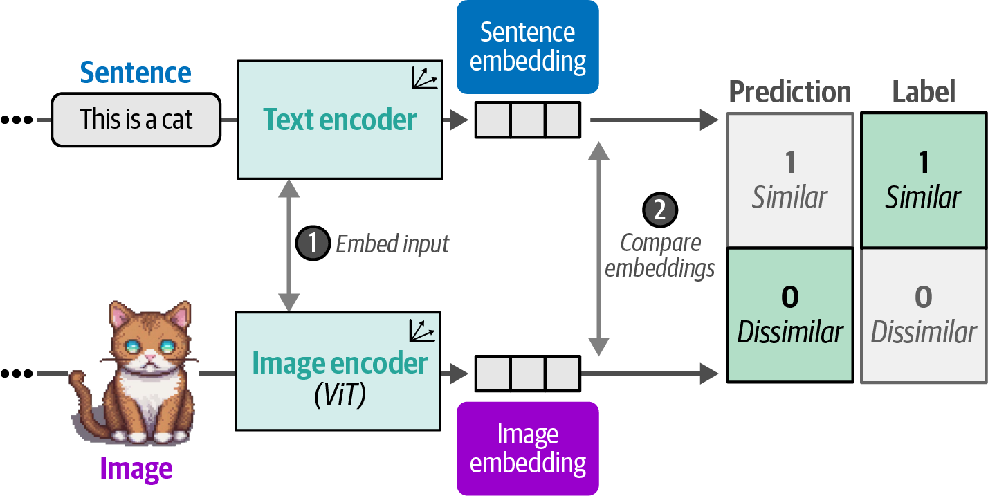
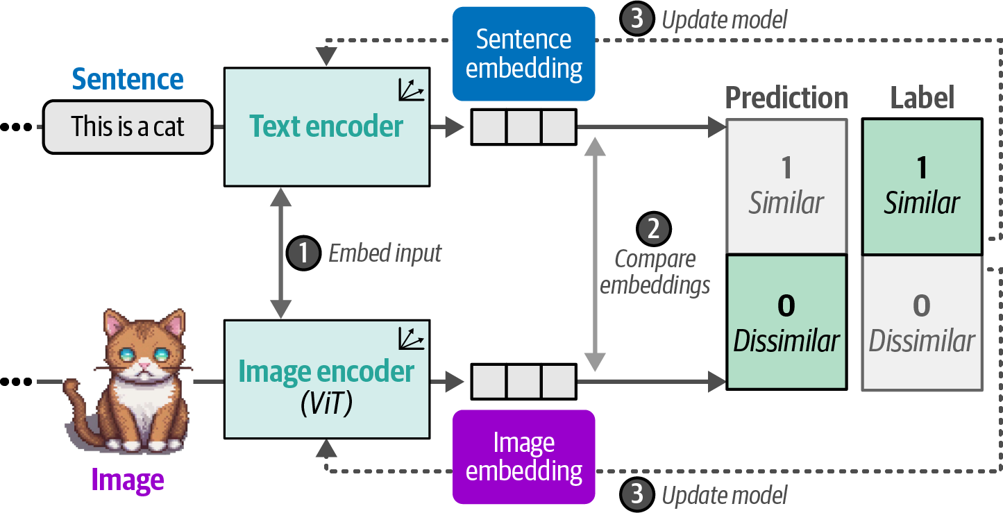
from urllib.request import urlopen
from PIL import Image

# load an AI-generated image of a puppy playing in the snow from a URL
puppy_path = (
    "https://raw.githubusercontent.com/"
    "HandsOnLLM/Hands-On-Large-Language-Models/main/"
    "chapter09/images/puppy.png"
)
# open the image from the URL and convert it to RGB format
image = Image.open(urlopen(puppy_path)).convert("RGB")
# define a text caption for the image
caption = "a puppy playing in the snow"
from transformers import CLIPTokenizer, CLIPProcessor, CLIPModel

model_id = "openai/clip-vit-base-patch32"

# load the tokenizer associated with the CLIP model to preprocess text
clip_tokenizer = CLIPTokenizer.from_pretrained(model_id, use_fast=True)

# load the processor associated with the CLIP model to preprocess images and text
clip_processor = CLIPProcessor.from_pretrained(model_id, use_fast=True)

# load the main CLIP model for generating text and image embeddings
model = CLIPModel.from_pretrained(model_id)
# tokenize the input caption into numerical representations
inputs = clip_tokenizer(caption, return_tensors="pt")
inputs{'input_ids': tensor([[49406, 320, 6829, 1629, 530, 518, 2583, 49407]]), 'attention_mask': tensor([[1, 1, 1, 1, 1, 1, 1, 1]])}# convert the token IDs back to the corresponding text tokens
clip_tokenizer.convert_ids_to_tokens(inputs["input_ids"][0])['<|startoftext|>',
'a</w>',
'puppy</w>',
'playing</w>',
'in</w>',
'the</w>',
'snow</w>',
'<|endoftext|>']# create a text embedding vector representing the semantic meaning of the caption
text_embedding = model.get_text_features(**inputs)
text_embedding.shape # (batch_size, embedding_dimension)torch.Size([1, 512])# preprocess the image to match the input requirements of the CLIP model
image_inputs = clip_processor(text=None, images=image, return_tensors="pt")
image_pixel_values = image_inputs["pixel_values"]
image_pixel_values.shape # (batch_size, num_channels, height, width)torch.Size([1, 3, 224, 224])import torch
import numpy as np
import matplotlib.pyplot as plt
# prepare the preprocessed image tensor for visualization
img = image_pixel_values.squeeze(0)
# remove the batch dimension
img = img.permute(*torch.arange(img.ndim - 1, -1, -1))
# transpose dimensions for correct visualization order (C, H, W -> H, W, C)
img = np.einsum("ijk->jik", img)
# visualize the preprocessed image
plt.imshow(img)
# turn off axis labels and ticks
plt.axis("off")
# create the image embedding vector representing the visual content of the image
image_embedding = model.get_image_features(image_pixel_values)
image_embedding.shape  # (batch_size, embedding_dimension): same as that of the text embedding
torch.Size([1, 512])# normalize the text and image embeddings
text_embedding /= text_embedding.norm(dim=-1, keepdim=True)
image_embedding /= image_embedding.norm(dim=-1, keepdim=True)
# calculate the cosine similarity score
text_embedding = text_embedding.detach().cpu().numpy()
# move the text embedding to CPU and convert to NumPy array
image_embedding = image_embedding.detach().cpu().numpy()
# move the image embedding to CPU and convert to NumPy array
score = np.dot(text_embedding, image_embedding.T)
scorearray([[0.33146894]], dtype=float32)|
|
9.3. Multimodal Text Generation Models
BLIP-2 (Bootstrapping Language-Image Pre-training for Unified Vision-Language Understanding and Generation 2) is a multimodal text generation model designed to introduce vision capabilities to existing, pre-trained language models (LLMs) without requiring end-to-end training from scratch.
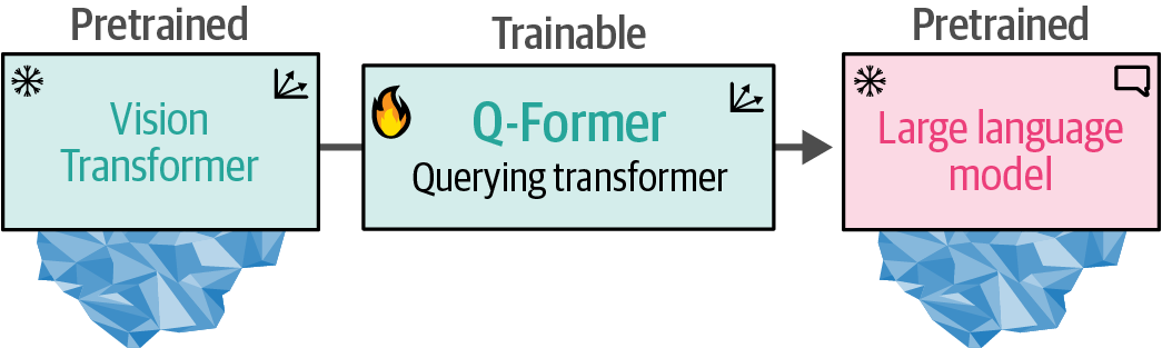
9.3.1. BLIP-2: Bridging the Modality Gap
BLIP-2 bridges the vision-language gap by building a bridge, named the Querying Transformer (Q-Former), connecting a frozen (non-trainable) pre-trained image encoder like a Vision Transformer and a frozen pre-trained LLM.
-
The Q-Former is trained in two stages, one for each modality to make it possible for the Q-Former to learn visual and textual representations in the same dimensional space, which can be used as a soft prompt to the LLM to give information about the image in a similar manner to the context providing an LLM when prompting.
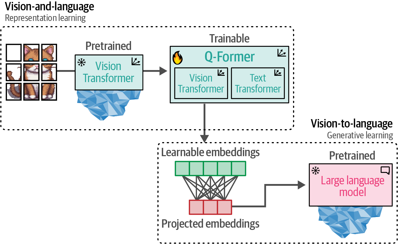 Figure 107. In step 1, representation learning is applied to learn representations for vision and language simultaneously. In step 2, these representations are converted to soft visual prompts to feed the LLM.
-
In step 1, image-document pairs are used to train the Q-Former to represent both images and text, which are generally captions of images similar tranning CLIP.
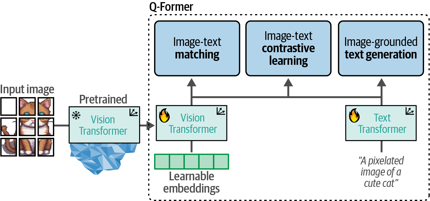 Figure 108. In step 1, the output of the frozen ViT is used together with its caption and trained on three contrastive-like tasks to learn visual-text representations.
-
The images are fed to the frozen ViT to extract vision embeddings, which are used as the input of Q-Former’s ViT, and the captions are used as the input of Q-Former’s Text Transformer.
-
The Q-Former is then trained on three tasks: image-text contrastive learning that attempts to align pairs of image and text embeddings such that they maximize their mutual information, image-text matching that predicts whether an image and text pair is positive (matched) or negative (unmatched), and image-grounded text generation that generates text based on information extracted from the input image.
-
-
In step 2, the learnable embeddings containing aligned visual and textual information in the same dimensional space from the Q-Former are projected to match the LLM’s input format and then serve as soft visual prompts, conditioning the LLM on the visual representations.
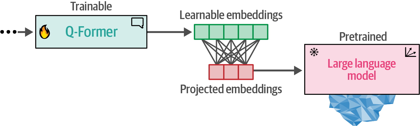 Figure 109. In step 2, the learned embeddings from the Q-Former are passed to the LLM through a projection layer. The projected embeddings serve as a soft visual prompt.
-
9.3.2. Preprocessing Multimodal Inputs
from urllib.request import urlopen

from PIL import Image

# load image of a supercar
car_path = (
    "https://raw.githubusercontent.com/"
    "HandsOnLLM/Hands-On-Large-Language-Models/main/"
    "chapter09/images/car.png"
)
with Image.open(urlopen(car_path)) as i:
    image = i.convert("RGB")
import torch
from transformers import AutoProcessor, Blip2ForConditionalGeneration

# load processor and main model
dev = "cuda" if torch.cuda.is_available() else "cpu"
model_id = "Salesforce/blip2-opt-2.7b"
blip_processor = AutoProcessor.from_pretrained(model_id, use_fast=True)
model = Blip2ForConditionalGeneration.from_pretrained(
    model_id,
    torch_dtype=torch.float16,
    device_map=dev,
)model.vision_model # vision transformer in the loaded BLIP-2 model.Blip2VisionModel(
(embeddings): Blip2VisionEmbeddings(
(patch_embedding): Conv2d(3, 1408, kernel_size=(14, 14), stride=(14, 14))
)
(encoder): Blip2Encoder(
(layers): ModuleList(
(0-38): 39 x Blip2EncoderLayer(
(self_attn): Blip2Attention(
(dropout): Dropout(p=0.0, inplace=False)
(qkv): Linear(in_features=1408, out_features=4224, bias=True)
(projection): Linear(in_features=1408, out_features=1408, bias=True)
)
(layer_norm1): LayerNorm((1408,), eps=1e-06, elementwise_affine=True)
(mlp): Blip2MLP(
(activation_fn): GELUActivation()
(fc1): Linear(in_features=1408, out_features=6144, bias=True)
(fc2): Linear(in_features=6144, out_features=1408, bias=True)
)
(layer_norm2): LayerNorm((1408,), eps=1e-06, elementwise_affine=True)
)
)
)
(post_layernorm): LayerNorm((1408,), eps=1e-06, elementwise_affine=True)
)model.language_model # text generative model in the loaded BLIP-2 model.OPTForCausalLM(
(model): OPTModel(
(decoder): OPTDecoder(
(embed_tokens): Embedding(50304, 2560, padding_idx=1)
(embed_positions): OPTLearnedPositionalEmbedding(2050, 2560)
(final_layer_norm): LayerNorm((2560,), eps=1e-05, elementwise_affine=True)
(layers): ModuleList(
(0-31): 32 x OPTDecoderLayer(
(self_attn): OPTSdpaAttention(
(k_proj): Linear(in_features=2560, out_features=2560, bias=True)
(v_proj): Linear(in_features=2560, out_features=2560, bias=True)
(q_proj): Linear(in_features=2560, out_features=2560, bias=True)
(out_proj): Linear(in_features=2560, out_features=2560, bias=True)
)
(activation_fn): ReLU()
(self_attn_layer_norm): LayerNorm((2560,), eps=1e-05, elementwise_affine=True)
(fc1): Linear(in_features=2560, out_features=10240, bias=True)
(fc2): Linear(in_features=10240, out_features=2560, bias=True)
(final_layer_norm): LayerNorm((2560,), eps=1e-05, elementwise_affine=True)
)
)
)
)
(lm_head): Linear(in_features=2560, out_features=50304, bias=False)
)# preprocess the image
image_inputs = blip_processor(image, return_tensors="pt").to(dev, torch.float16)
image_pixel_values = image_inputs["pixel_values"]
image_pixel_values.shape # a 224 × 224-sized imagetorch.Size([1, 3, 224, 224])# tokenizer used to tokenize the input text
blip_processor.tokenizerGPT2TokenizerFast(name_or_path='Salesforce/blip2-opt-2.7b', vocab_size=50265, model_max_length=1000000000000000019884624838656, is_fast=True, padding_side='right', truncation_side='right', special_tokens={'bos_token': '</s>', 'eos_token': '</s>', 'unk_token': '</s>', 'pad_token': '<pad>'}, clean_up_tokenization_spaces=False, added_tokens_decoder={
1: AddedToken("<pad>", rstrip=False, lstrip=False, single_word=False, normalized=True, special=True),
2: AddedToken("</s>", rstrip=False, lstrip=False, single_word=False, normalized=True, special=True),
50265: AddedToken("<image>", rstrip=False, lstrip=False, single_word=False, normalized=False, special=True),
}
)# preprocess the text
text = "Her vocalization was remarkably melodic"
token_ids = blip_processor(image, text=text, return_tensors="pt")
token_ids = token_ids.to(dev, torch.float16)["input_ids"][0]
# convert input ids back to tokens
tokens = blip_processor.tokenizer.convert_ids_to_tokens(token_ids)
tokens['</s>', 'Her', 'Ġvocal', 'ization', 'Ġwas', 'Ġremarkably', 'Ġmel', 'odic']# replace the space token with an underscore
tokens = [token.replace("Ġ", "_") for token in tokens]
tokens['</s>', 'Her', '_vocal', 'ization', '_was', '_remarkably', '_mel', 'odic']9.3.3. Use Case 1: Image Captioning
from urllib.request import urlopen

import torch
from PIL import Image
from transformers import AutoProcessor, Blip2ForConditionalGeneration

# load processor and main model
dev = "cuda" if torch.cuda.is_available() else "cpu"
dtype = torch.float16 if torch.cuda.is_available() else torch.float32

model_id = "Salesforce/blip2-opt-2.7b"
blip_processor = AutoProcessor.from_pretrained(model_id, use_fast=True)
model = Blip2ForConditionalGeneration.from_pretrained(
    model_id,
    torch_dtype=dtype,
    device_map=dev,
)

# load an AI-generated image of a supercar
car_path = (
    "https://raw.githubusercontent.com/"
    "HandsOnLLM/Hands-On-Large-Language-Models/main/"
    "chapter09/images/car.png"
)
with Image.open(urlopen(car_path)) as i:
    image = i.convert("RGB")

# convert an image into inputs and preprocess it
inputs = blip_processor(image, return_tensors="pt").to(dev, dtype)
# {'pixel_values': tensor([[[[-1.0039, -1.0039, -0.9893,  ..., -0.0842, -0.0988, -0.0842],

# generate image ids to be passed to the decoder (LLM)
generated_ids = model.generate(**inputs, max_new_tokens=20)

# generate text from the image ids
generated_text = blip_processor.batch_decode(
    generated_ids, skip_special_tokens=True
)
generated_text = generated_text[0].strip()
generated_text
an orange supercar driving on the road at sunset9.3.4. Use Case 2: Multimodal Chat-Based Prompting
from urllib.request import urlopen

import torch
from PIL import Image
from transformers import AutoProcessor, Blip2ForConditionalGeneration

# load processor and main model
dev = "cuda" if torch.cuda.is_available() else "cpu"
dtype = torch.float16 if torch.cuda.is_available() else torch.float32

model_id = "Salesforce/blip2-opt-2.7b"
blip_processor = AutoProcessor.from_pretrained(model_id, use_fast=True)
model = Blip2ForConditionalGeneration.from_pretrained(
    model_id,
    torch_dtype=dtype,
    device_map=dev,
)

# load an AI-generated image of a supercar
car_path = (
    "https://raw.githubusercontent.com/"
    "HandsOnLLM/Hands-On-Large-Language-Models/main/"
    "chapter09/images/car.png"
)
with Image.open(urlopen(car_path)) as i:
    image = i.convert("RGB")

# visual question answering
prompt = "Question: Write down what you see in this picture. Answer:"

# process both the image and the prompt
inputs = blip_processor(image, text=prompt, return_tensors="pt").to(dev, dtype)

# generate text
generated_ids = model.generate(**inputs, max_new_tokens=30)
generated_text = blip_processor.batch_decode(
    generated_ids, skip_special_tokens=True
)
generated_text = generated_text[0].strip()
generated_text
Question: Write down what you see in this picture. Answer: A sports car driving on the road at sunset# chat-like prompting: a follow-up question
prompt = (
"Question: Write down what you see in this picture. Answer: A sports "
"car driving on the road at sunset. Question: What would it cost me to "
"drive that car? Answer:"
)
# Generate output
inputs = blip_processor(image, text=prompt, return_tensors="pt").to(dev, dtype)
generated_ids = model.generate(**inputs, max_new_tokens=30)
generated_text = blip_processor.batch_decode(
generated_ids, skip_special_tokens=True
)
generated_text = generated_text[0].strip()
generated_textQuestion: Write down what you see in this picture. Answer: A sports car driving on the road at sunset. Question: What would it cost me to drive that car? Answer: $1,000,00010. Creating and Fine-Tuning Text Embedding Models
Embedding models are Large Language Models (LLMs) used to convert unstructured textual data (like documents, sentences, or phrases) into dense numerical representations called embeddings.
-
The primary goal of these models is to accurately capture the semantic meaning of the text, such that texts with similar meanings have embeddings that are close to each other in a high-dimensional vector space, while texts with different meanings have dissimilar embeddings.
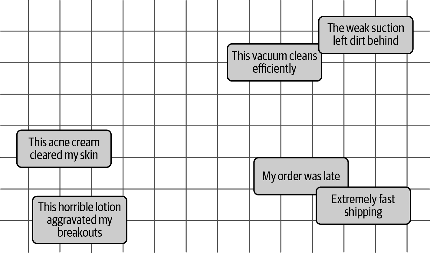 Figure 111. The idea of semantic similarity is that we expect textual data with similar meanings to be closer to each other in n-dimensional space (two dimensions are illustra‐ ted here).
 -
Embedding models can also be trained or fine-tuned for other purposes, such as capturing sentiment similarity, by guiding the model with appropriate training examples.
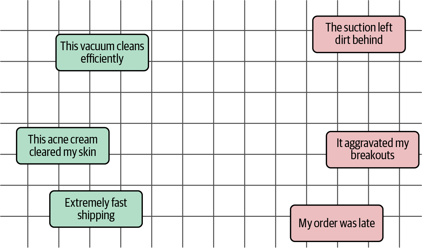 Figure 112. In addition to semantic similarity, an embedding model can be trained to focus on sentiment similarity. In this figure, negative reviews (red) are close to one another and dissimilar to positive reviews (green).
10.1. Contrastive Learning
Contrastive learning is a self-supervised or supervised machine learning technique that aims to learn representations of data by contrasting similar ("positive") and dissimilar ("negative") examples (Why P and not Q?) to create an embedding space where similar data points are located close to each other, while dissimilar data points are far apart, which is effective in various domains, including computer vision and natural language processing, for tasks like representation learning, similarity search, and few-shot learning.
Reporter: “Why did you rob a bank?”

Robber: “Because that is where the money is.”

Reporter (alternatively): “Why did you rob a bank (P) instead of obeying the law (Q)?”
10.2. Sentence Transformers (SBERT)
A cross-encoder is a Transformer-based model that processes two sentences together to directly predict their similarity score via a classification head, but it’s computationally expensive for large-scale pairwise comparisons and doesn’t typically generate individual sentence embeddings.
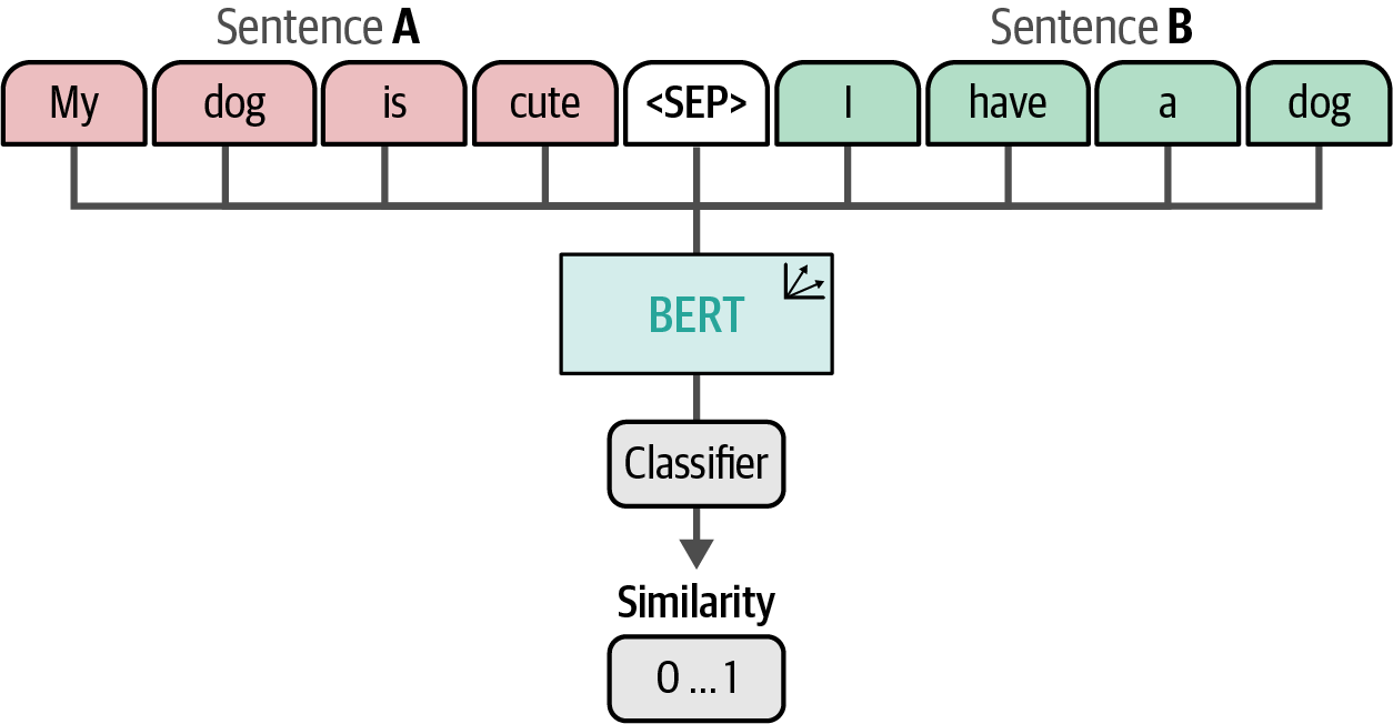
The authors of sentence-transformers addressed the limitations of cross-encoders (slow speed, no embeddings) by developing a fast alternative that generates semantically comparable, fixed-size embeddings by using a Siamese architecture, also known as a bi-encoder or SBERT, with two identical BERT models (sharing weights) that process sentences independently and then apply mean pooling to the final layer.
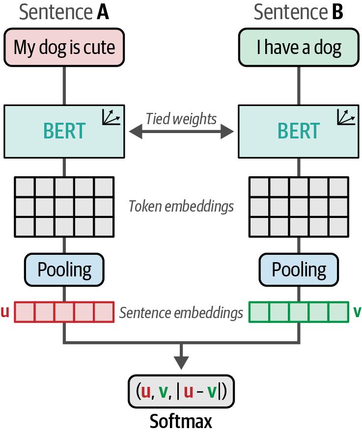
10.3. Creating an Embedding Model
Natural Language Inference (NLI) datasets, used in pretraining embedding models, classify premise-hypothesis pairs as entailment (similar meaning), contradiction (opposite meaning), or neutral.
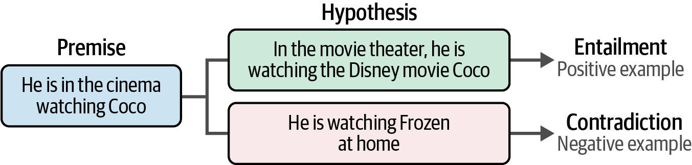
-
Entailments serve as positive examples for contrastive learning (similar pairs), while contradictions serve as negative examples (dissimilar pairs).
-
The Multi-Genre Natural Language Inference (MNLI) corpus from the General Language Understanding Evaluation (GLUE) benchmark contains annotated sentence pairs with these relationships, and is a common source for generating such contrastive training data.
-
A subset of MNLI is often used for faster experimentation, though larger, quality datasets are generally preferred for stable training.
from datasets import load_dataset # Load MNLI dataset from GLUE # 0 = entailment, 1 = neutral, 2 = contradiction train_dataset = load_dataset( "glue", # load a dataset from the GLUE benchmark "mnli", # load the MNLI dataset split="train", # load the training split ).select(range(50_000)) train_dataset = train_dataset.remove_columns("idx")train_dataset[2]{'premise': 'One of our number will carry out your instructions minutely.', 'hypothesis': 'A member of my team will execute your orders with immense precision.', 'label': 0}
# train model
from sentence_transformers import SentenceTransformer

# use a base model
model = SentenceTransformer("google-bert/bert-base-uncased")

from sentence_transformers import losses

# define the softmax loss function.
train_loss = losses.SoftmaxLoss(
    model=model,
    sentence_embedding_dimension=model.get_sentence_embedding_dimension(),
    num_labels=3,
)

from sentence_transformers.evaluation import EmbeddingSimilarityEvaluator

# create an embedding similarity evaluator for STSB
val_sts = load_dataset("glue", "stsb", split="validation")
evaluator = EmbeddingSimilarityEvaluator(
    sentences1=val_sts["sentence1"],
    sentences2=val_sts["sentence2"],
    scores=[score / 5 for score in val_sts["label"]],
    main_similarity="cosine",
)

from sentence_transformers.training_args import (
    SentenceTransformerTrainingArguments,
)

args = SentenceTransformerTrainingArguments(
    output_dir="base_embedding_model",
    num_train_epochs=1,
    per_device_train_batch_size=32,
    per_device_eval_batch_size=32,
    warmup_steps=100,
    fp16=True,
    eval_steps=100,
    logging_steps=100,
)

from sentence_transformers.trainer import SentenceTransformerTrainer

# train embedding model
trainer = SentenceTransformerTrainer(
    model=model,
    args=args,
    train_dataset=train_dataset,
    loss=train_loss,
    evaluator=evaluator,
)
trainer.train()

# evaluate the trained model
evaluator(model)