
- 1. What is Data Engineering?
- 2. Data Warehouses, Lakes, and Lakehouses
- 3. Data Architecture
- 4. Data Sources
- 5. Data Storage Systems
- 6. Data Ingestion
- 7. Data Transformation
- 8. Data Serving
- 9. Data Serving for Analytics and ML
- 10. Reverse ETL
- Appendix A: Serialization and Compression
- References
1. What is Data Engineering?
Data engineering is the development, implementation, and maintenance of systems and processes that take in raw data and produce high-quality, consistent information that supports downstream use cases, such as analysis and machine learning, while is also the intersection of security, data management, DataOps, data architecture, orchestration, and software engineering.
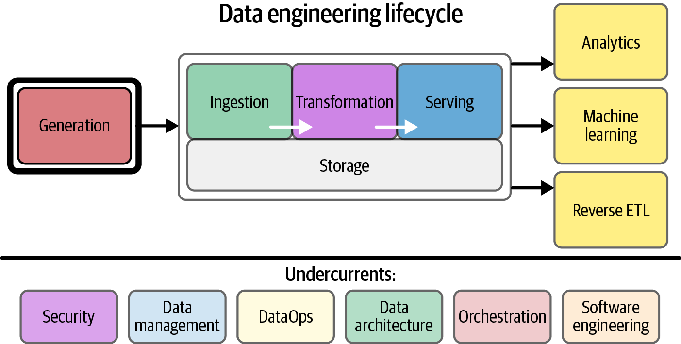
| A data engineer manages the data engineering lifecycle, beginning with getting data from source systems and ending with serving data for use cases, such as analysis or machine learning. |
1.1. DataOps
DataOps applies Agile, DevOps, and statistical process control to data, aiming to improve the release and quality of data products by reducing time to value, which is a cultural shift emphasizing collaboration, continuous learning, and rapid iteration, supported by three core technical elements:
-
automation (for reliability, consistency, and CI/CD)
-
monitoring and observability (including the Data Observability Driven Development (DODD) method for end-to-end data visibility to prevent issues)
-
incident response (to rapidly identify and resolve problems).
| DataOps seeks to proactively address issues, build trust, and continuously improve data engineering workflows, despite the current immaturity of data operations compared to software engineering. |
1.2. ETL and ELT
ETL (extract, transform, load) is the traditional data warehouse approach where the extract phase pulls data from source systems, the transform phase cleans and standardizes data while organizing and imposing business logic in a highly modeled form, and the load phase pushes the transformed data into the data warehouse target database system, and the processes are typically handled by external systems and work hand-in-hand with specific business structures and teams.
ELT (extract, load, transform) is a variation where data is moved more directly from production systems into a staging area in the data warehouse in raw form, and transformations are handled directly within the data warehouse itself rather than using external systems, that takes advantage of the massive computational power of cloud data warehouses and data processing tools, with data processed in batches and transformed output written into tables and views for analytics.
2. Data Warehouses, Lakes, and Lakehouses
Data could be stored and managed through distinct architectural approaches for analytical purposes: data warehouses are highly structured and optimized for reporting, data lakes store raw and diverse data, while data lakehouses merge the flexibility of data lakes with the robust management features of data warehouses.
2.1. Data Warehouses
A data warehouse is a central data hub designed for reporting and analysis, characterized as a subject-oriented, integrated, nonvolatile, and time-variant collection of data that supports management decisions.
-
A data warehous separates online analytical processing (OLAP) from production databases and centralizes data through ETL (extract, transform, load) or ELT (extract, load, transform) processes, organizing data into highly formatted structures optimized for analytics.
-
A data mart is a refined subset of a data warehouse specifically designed to serve the analytics and reporting needs of a single suborganization, department, or line of business, that makes data more accessible to analysts and provide an additional transformation stage beyond initial ETL/ELT pipelines, improving performance for complex queries by pre-joining and aggregating data.
A cloud data warehouse represents a significant evolution from on-premises architectures, pioneered by Amazon Redshift and popularized by Google BigQuery and Snowflake, which offers pay-as-you-go scalability, separates compute from storage using object storage for virtually limitless capacity, and can process petabytes of data in single queries.
-
A cloud data warehouse has expanded MPP capabilities to cover big data use cases that previously required Hadoop clusters, blurring the line between traditional data warehouses and data lakes while evolving into broader data platforms with enhanced capabilities.
-
A cloud data warehous cannot handle truly unstructured data, such as images, video, or audio, unlike a true data lake, but can be coupled with object storage to provide a complete data-lake solution.
2.2. Data Lakes
A data lake is a central repository that stores all data—structured, semi-structured, and unstructured—in its raw format with virtually limitless capacity, emerging during the big data era as an alternative to structured data warehouses that promised democratized data access and flexible processing using technologies like Spark, but first-generation data lake 1.0 became known as a "data swamp" due to lack of schema management, data cataloging, and discovery tools, while being write-only and creating compliance issues with regulations like GDPR, CCPA etc.
2.3. Data Lakehouses
A data lakehouse represents a convergence between data lakes and data warehouses, incorporating the controls, data management, and data structures found in data warehouses while still housing data in object storage and supporting various query and transformation engines, with ACID transaction support that addresses the limitations of first-generation data lakes by providing proper data management capabilities instead of the original write-only approach.
-
A lakehouse system is a metadata and file-management layer deployed with data management and transformation tools.
-
Databricks has heavily promoted the lakehouse concept with Delta Lake, an open source storage management system.
3. Data Architecture
Lambda, Kappa, and Dataflow are distinct architectural patterns for designing data processing systems, each offering approaches to manage and unify both batch and real-time data streams.
3.1. Lambda Architecture
Lambda architecture is a data processing architecture that handles both batch and streaming data through three independent systems: a batch layer that processes historical data in systems like data warehouses, a speed layer that processes real-time data with low latency using NoSQL databases, and a serving layer that combines results from both layers, though it faces challenges with managing multiple codebases and reconciling data between systems.
3.2. Kappa Architecture
Kappa architecture is an alternative to Lambda that uses a stream-processing platform as the backbone for all data handling—ingestion, storage, and serving—enabling both real-time and batch processing on the same data by reading live event streams and replaying large chunks for batch processing, though it hasn’t seen widespread adoption due to streaming complexity and cost compared to traditional batch processing.
3.3. Dataflow Model
The Dataflow model, developed by Google and implemented through Apache Beam, addresses the challenge of unifying batch and streaming data by viewing all data as events where aggregation is performed over various windows, treating real-time streams as unbounded data and batches as bounded event streams, enabling both processing types to happen in the same system using nearly identical code through the philosophy of "batch as a special case of streaming," which has been adopted by frameworks like Flink and Spark.
3.4. IoT
IoT (Internet of Things) devices are physical hardware that sense their environment and collect/transmit data, connected through IoT gateways that serve as hubs for data retention and internet routing, with ingestion flowing into event architectures that vary from real-time streaming to batch uploads depending on connectivity, storage requirements ranging from batch object storage for remote sensors to message queues for real-time responses, and serving patterns spanning from batch reports to real-time anomaly detection with reverse ETL patterns where analyzed sensor data is sent back to reconfigure and optimize manufacturing equipment.
4. Data Sources
4.1. OLTP and OLAP
An Online Transactional Processing (OLTP) data system is designed as an application database to store the state of an application, typically supporting atomicity, consistency, isolation, and durability as part of ACID characteristics, but not ideal for large-scale analytics or bulk queries.
In contrast, an online analytical processing (OLAP) system is designed for large-scale, interactive analytics queries, but making it inefficient for single record lookups but enabling its use as a data source for machine learning models or reverse ETL workflows, while the online part implies the system constantly listens for incoming queries.
4.2. Message Queues and Event-Streaming
A message is a discrete piece of raw data communicated between systems, which is typically removed from a queue once it’s delivered and consumed, while a stream is an append-only, ordered log of event records that are persisted over a longer duration to allow for complex analysis of what happened over many events.
While time is an essential consideration for all data ingestion, it becomes that much more critical and subtle in the context of streaming, where
-
event time is when an event is generated at the source;
-
ingestion time is when it enters a storage system like a message queue, cache, memory, object storage, or a database;
-
process time is when it undergoes transformation; and
-
processing time measures how long that transformation took, measured in seconds, minutes, hours, etc.
Event-driven architectures, critical for data apps and real-time analytics, leverage message queues and event-streaming platforms, which can serve as source systems and span the data engineering lifecycle.
-
Message queues asynchronously send small, individual messages between decoupled systems using a publish/subscribe model, buffering messages, ensuring durability, and handling delivery frequency (exactly once or at least once), though message ordering can be fuzzy in distributed systems.
-
Event-streaming platforms are a continuation of message queues but primarily ingest and process data as an ordered, replayable log of records (events with key, value, timestamp), organized into topics (collections of related events) and subdivided into stream partitions for parallelism and fault tolerance, with careful partition key selection needed to avoid hotspotting.
4.3. Relational Databases and Nonrelational Databases
A Relational Database Management System (RDBMS) stores data in tables of relations (rows) with fields (columns), typically indexed by a primary key and supporting foreign keys for joins, and is popular, ACID compliant, and ideal for storing rapidly changing application states, often employing normalization to prevent data duplication.
NoSQL, or not only SQL, databases emerged as alternatives to relational systems, offering improved performance, scalability, and schema flexibility by abandoning traditional RDBMS constraints like strong consistency, joins, or fixed schemas; they encompass diverse types such as key-value, document, wide-column, graph, search, and time series, each tailored for specific workloads.
-
A key-value database is a nonrelational database that uniquely identifies and retrieves records using a key, similar to a hash map but more scalable, offering diverse performance characteristics for use cases ranging from high-speed, temporary caching to durable persistence for massive event state changes.
-
A document store, a specialized key-value database, organizes nested objects (documents, often JSON-like) into collections for key-based retrieval; while offering schema flexibility, it is typically not ACID compliant and lacks joins, promoting denormalization, and is often eventually consistent.
-
A wide-column database is optimized for massive data storage, high transaction rates, and low latency, scaling to petabytes and millions of requests per second, making them popular in various industries; however, they only support rapid scans with a single row key index, necessitating data extraction to secondary analytics systems for complex queries. Note that wide-column refers to the database’s architecture, allowing flexible and sparse columns per row, which is distinct from a wide table, a denormalized data modeling concept with many columns.
-
A graph database explicitly stores data with a mathematical graph structure (nodes and edges), making them ideal for analyzing connectivity and complex traversals between elements, unlike other databases that struggle with such queries; it utilizes specialized query languages and present unique challenges for data engineers in terms of data mapping and analytics tool adoption.
-
A search database is a nonrelational database optimized for fast search and retrieval of complex and simple semantic and structural data, primarily used for text search (exact, fuzzy, or semantic matching) and log analysis (anomaly detection, real-time monitoring, security, and operational analytics), often leveraging indexes for speed.
-
A time-series database is optimized for retrieving and statistically processing time-ordered data, handling high-velocity, often write-heavy workloads (including regularly generated measurement data and irregularly created event-based data) by utilizing memory buffering for fast writes and reads; its timestamp-ordered schema makes it suitable for operational analytics, though generally not for BI due to a typical lack of joins.
4.4. APIs
APIs are standard for data exchange in the cloud and between systems, with HTTP-based APIs being most popular.
-
REST (Representational State Transfer) is a dominant, stateless API paradigm built around HTTP verbs, though it lacks a full specification and requires domain knowledge.
-
GraphQL is an alternative query language that allows retrieving multiple data models in a single request, offering more flexibility than REST.
-
Webhooks are event-based, reverse APIs where the data source triggers an HTTP endpoint on the consumer side when specified events occur.
-
RPC (Remote Procedure Call) allows running procedures on remote systems; gRPC, developed by Google, is an efficient RPC library built on Protocol Buffers for bidirectional data exchange over HTTP/2.
5. Data Storage Systems
Distributed systems navigate a fundamental trade-off between performance and data integrity, where systems built on the ACID model guarantee strong consistency for data correctness at the cost of higher latency, while those following the BASE model favor high availability and scalability through eventual consistency, which tolerates temporary data staleness.
5.1. File Storage and Block Storage
File storage systems—whether local (like NTFS and ext4), network-attached (NAS), storage area network (SAN), or cloud-based (like Amazon EFS)—organize data into directory trees with specific read/write characteristics; however, for modern data pipelines, object storage, such as Amazon S3, is often the preferred approach.
Block storage, the raw storage provided by disks and virtualized in the cloud, offers fine-grained control and is fundamental for transactional databases and VM boot disks, with solutions like RAID, SAN, and cloud-specific offerings (e.g., Amazon EBS) providing varying levels of performance, durability, and features, alongside local instance volumes for high-performance, ephemeral caching.
-
A block is the smallest addressable unit of data supported by a disk, typically 4,096 bytes on modern disks, containing extra bits for error detection/correction and metadata.
-
On magnetic disks, blocks are geometrically arranged, and reading blocks on different tracks requires a "seek," a time-consuming operation that is negligible on SSDs.
-
RAID (Redundant Array of Independent Disks) controls multiple disks to improve data durability, enhance performance, and combine capacity, appearing as a single block device to the operating system.
-
SAN (Storage Area Network) systems provide virtualized block storage devices over a network, offering fine-grained scaling, enhanced performance, availability, and durability.
-
Cloud virtualized block storage solutions, like Amazon EBS, abstract away SAN clusters and networking, providing various tiers of service with different performance characteristics (IOPS and throughput), backed by SSDs for higher performance or magnetic disks for lower cost per gigabyte.
-
Local instance volumes are block storage physically attached to the host server running a VM, offering low cost, low latency, and high IOPS, but their data is lost when the VM shuts down or is deleted, and they lack advanced virtualization features like replication or snapshots.
5.2. Object Storage
Object storage, a key-value store for immutable data objects (like files, images, and videos) popular in big data and cloud environments (e.g., Amazon S3), offers high performance for parallel reads/writes, scalability, durability, and various storage tiers, but lacks in-place modification and true directory hierarchies, making it ideal for data lakes and ML pipelines despite consistency and versioning complexities.
-
Object storage is a key-value store for immutable data objects (files like TXT, CSV, JSON, images, videos, audio) that has gained popularity with big data and cloud computing (e.g., Amazon S3, Azure Blob Storage, Google Cloud Storage).
-
Objects are written once as a stream of bytes and become immutable; changes require rewriting the full object.
-
Object stores support highly performant parallel stream writes and reads, scaling with the number of streams and virtual machines, making them ideal for high-volume web traffic and distributed query engines.
-
Cloud object storage offers high durability and availability by saving data in multiple availability zones, with various storage classes available at discounted prices for reduced access or durability.
-
Object stores are a key ingredient in separating compute and storage, enabling ephemeral clusters and virtually limitless, scalable storage.
-
For data engineering, object stores excel at large batch reads and writes, serving as the gold standard for data lakes, and are suitable for unstructured data in ML pipelines.
-
Object lookup relies on a top-level logical container (bucket) and a key, lacking a true directory hierarchy; consequently, "directory"-level operations can be costly due to the need for key prefix filtering.
-
Object consistency can be eventual or strong (latter often achieved with an external database), and object versioning allows retaining previous immutable versions, though at an increased storage cost.
-
Lifecycle policies allow automatic deletion of old versions or archiving to cheaper tiers.
-
Object store-backed filesystems (e.g., s3fs, Amazon S3 File Gateway) allow mounting object storage as local storage, but are best suited for infrequently updated files due to the immutability of objects.
5.3. HDFS
The Hadoop Distributed File System (HDFS), based on Google File System (GFS), is a distributed storage system that breaks large files into blocks managed by a NameNode, with data replicated across multiple nodes for durability and availability, and it combines compute and storage on the same nodes, unlike object stores.
-
HDFS breaks large files into blocks (less than a few hundred megabytes), managed by a NameNode that maintains directories, file metadata, and block locations.
-
Data is typically replicated to three nodes for high durability and availability; the NameNode ensures replication factor is maintained.
-
HDFS combines compute resources with storage nodes, originally for the MapReduce programming model, allowing in-place data processing.
-
While some Hadoop ecosystem tools are declining, HDFS remains widely used in legacy installations and as a key component in current big data engines like Amazon EMR, often running with Apache Spark.
5.4. Indexes, Partitioning, and Clustering
Indexes, partitioning, and clustering are database optimization techniques that have evolved from traditional row-oriented indexing to columnar storage, enabling efficient analytical queries through data organization and pruning.
-
Indexes provide a map of the table for particular fields and allow extremely fast lookup of individual records.
-
Columnar databases store data by column, enabling faster scans for analytical queries by reading only relevant columns and achieving high compression ratios; while historically poor for joins, their performance has significantly improved.
-
Partitioning divides a table into smaller subtables based on a field (e.g., date-based partitioning) to reduce the amount of data scanned for a query.
-
Clustering organizes data within partitions by sorting it based on one or more fields, co-locating similar values to improve performance for filtering, sorting, and joining.
-
Snowflake Micro-partitioning is an advanced approach where data is automatically clustered into small, immutable units (50-500 MB) based on repeated values across fields, allowing aggressive query pruning using metadata that describes each micro-partition’s contents.
5.5. Data Catalog
A data catalog is a centralized metadata inventory that provides a unified, searchable view of all organizational data by automatically scanning sources like data lakes and warehouses to collect and infer metadata, including lineage, and serves a dual purpose: technically, it enables automated data discovery for applications like data lakehouses, while organizationally, it offers a collaborative portal for users to find, understand, and document data assets.
5.6. Separation of Compute and Storage
The separation of compute and storage is a foundational architectural pattern in the modern cloud, which diverges from the traditional colocation of these resources by capitalizing on the economic scalability of ephemeral compute and the enhanced durability of object storage. Because pure separation can introduce performance bottlenecks, a hybrid approach is frequently employed, manifesting as multi-tier caching where local storage accelerates processing, or as hybrid object storage that integrates compute functions directly.
5.7. Data Storage Lifecycle and Data Retention
The data storage lifecycle is a framework that manages data by categorizing it as hot, warm, or cold based on access frequency, which dictates its automated placement across corresponding storage tiers to optimize cost, which is complemented by data retention policies that determine the data’s lifespan by balancing its intrinsic value against storage costs and compliance mandates.
6. Data Ingestion
Data ingestion is the process of moving data from a source into a storage system. It is distinct from data integration, which combines data from multiple sources, and from internal data movement within a system, which is considered part of the transformation process.
A data pipeline is the combination of architecture, systems, and processes that move data through the stages of the data engineering lifecycle. Modern data pipelines are flexible and technology-agnostic, encompassing various patterns like ETL, ELT, and reverse ETL to suit the specific task, rather than adhering to a rigid philosophy.
6.1. Engineering
When designing a data ingestion system, key engineering considerations include understanding the data’s use case, destination, update frequency, volume, format, and quality. It’s also crucial to evaluate architectural factors such as whether the data is bounded or unbounded, the ingestion frequency (synchronous vs. asynchronous), serialization methods, throughput, reliability, payload size, and the data movement pattern (push, pull, or poll).
-
Bounded vs. Unbounded Data: Data is fundamentally unbounded, representing a continuous flow of events as they occur in reality, while bounded data is a practical bucketing of this flow within a defined boundary, such as a time window. Although business processes have historically imposed artificial bounds by creating discrete batches, modern streaming ingestion systems are designed to preserve the inherently unbounded nature of data, allowing for continuous processing throughout its lifecycle.
-
Frequency: The frequency of data ingestion spans a wide spectrum from slow batch processes to near real-time streaming, where "real-time" is a practical term for systems with very low latency, and these streaming systems, ideal for event-driven sources like IoT, often coexist with and feed into downstream batch processes, at which point the batch frequency becomes a bottleneck for all subsequent operations.
-
Synchronous and Asynchronous Ingestion: Synchronous ingestion creates tightly coupled workflows where each stage depends directly on the previous one, making the entire process prone to failure if any single step fails, whereas asynchronous ingestion decoupples these stages, allowing individual events to be processed in parallel as they become available, often using a buffer to manage load and increase resilience.
-
Serialization and Deserialization: This process involves encoding (serialization) data for transmission and requires ensuring the destination system can properly decode (deserialization) the received data to prevent it from becoming inert and unusable.
-
Throughput and Scalability: To prevent ingestion from becoming a bottleneck as data volumes change, systems must be designed for flexible scaling, incorporating buffering to handle bursty data rates and backlogs from source system downtime, while leveraging managed services is highly recommended to automate this complex scaling process.
-
Reliability and Durability: This involves ensuring high uptime with proper failover (reliability) to prevent data from being lost or corrupted (durability), a critical consideration given that the ingestion system’s reliability directly impacts the permanence of data from ephemeral sources, necessitating a risk-based approach to building appropriate levels of redundancy and self-healing.
-
Payload: The ingested dataset itself, whose characteristics—including its kind, shape, size, schema, and metadata—fundamentally determine how it must be handled throughout the entire data engineering lifecycle.
-
Kind: The data’s fundamental type (e.g., tabular, image, text) and its specific format (e.g., CSV, Parquet, JPG), which are directly linked as the type influences the format, and each format has distinct byte patterns requiring specific serialization and deserialization methods.
-
Shape: The specific dimensions of a payload, a critical characteristic that must be compatible with downstream systems, which varies by data kind, for example, the number of rows and columns for tabular data; the key-value pairs and nesting depth for JSON; the number of words or characters for unstructured text; the width, height, and color depth for images; and the number of channels, sample depth, and sample rate for audio.
-
Size: The payload’s byte size, which can range from single bytes to terabytes and is often managed by either compressing the data or by splitting a massive payload into smaller, more manageable chunks to facilitate easier and more reliable network transmission before being reassembled at the destination.
-
Schema and Data Types: The structure describing the fields and their corresponding data types within a payload, which presents a primary engineering challenge in understanding the organization of data in complex source systems, including those generated by ORMs and exposed by APIs.
-
Schema Evolution: Source system schemas frequently change (e.g., adding columns, changing types), which can break downstream pipelines. While automated detection and updates are increasingly common, they are a mixed blessing, as changes can still have adverse effects, necessitating robust strategies for both automated handling and clear communication with data consumers.
-
Schema Registries: In streaming systems where schemas constantly evolve, a schema registry acts as a metadata repository to maintain data type integrity, track schema versions, and ensure consistent serialization and deserialization between producers and consumers.
-
Metadata: The descriptive data about the payload—encompassing its schema, format, shape, and other characteristics—which is as critical as the data itself for providing the context and usability that were notably absent in early, failed data lake implementations.
-
-
-
Push vs. Pull vs. Poll: These patterns describe the data flow between systems, where a push strategy involves the source sending data to the target, a pull strategy involves the target retrieving data from the source, and a polling strategy involves the target periodically checking the source for changes and then pulling the data.
6.2. Batch
Batch ingestion, which involves processing data in bulk, is a convenient method where a subset of data is ingested from a source system based on either a specific time interval or the accumulated size of the data.
-
Time-interval batch ingestion is a widespread pattern in traditional ETL for data warehousing, often running daily during off-hours, while size-based batch ingestion is common for moving data from streaming systems into object storage for data lakes.
-
Common batch ingestion patterns include snapshot or differential extraction, file-based transfers, ETL/ELT processes, and data migration.
-
Snapshot or Differential Extraction involves choosing between capturing the entire current state of a source system (full snapshot) or only the changes since the last read (differential update), where differential updates minimize network and storage usage but full snapshots are often preferred for their simplicity.
-
File-Based Export and Ingestion is a push-based pattern where data is serialized into files on the source system and then transferred to the target via methods like object storage or SFTP, a technique that enhances security by avoiding direct database access and giving source system owners full control over data preprocessing and export.
-
ETL and ELT are common batch workload patterns, where Extract involves getting data from a source (via push or pull) while being mindful of metadata, and Load involves placing that data into a destination, with careful consideration of the target system’s type, schema, and performance impacts.
The key difference between ETL and ELT is where the transformation happens. In ETL, data is transformed before it’s loaded into the data warehouse, typically in a separate processing server. In ELT, raw data is loaded directly into the data warehouse first, and the transformation is then performed within the warehouse itself.
-
Inserts, Updates, and Batch Size is a critical consideration as many batch-oriented systems, particularly columnar databases, perform poorly with many small operations (like single-row inserts) that create suboptimal files, making it essential to understand the ideal update patterns and batch sizes for the specific data store to avoid performance degradation.
-
Data Migration involves moving data in bulk to a new database or environment, a process where careful schema management is crucial due to subtle differences between systems, and where the primary challenge often lies in redirecting data pipeline connections rather than the data movement itself.
-
6.3. Message and Stream
Ingesting event data is a common practice that requires careful consideration of several key issues, including schema evolution, late-arriving data, ordering and delivery guarantees, replay capabilities, time-to-live, message size, error handling with dead-letter queues, consumer push and pull models, and the physical location of the infrastructure.
-
Schema Evolution is a common challenge in handling event data, as changes in fields or value types can have unintended downstream impacts. To mitigate these issues, it is recommended to use a schema registry to version changes, employ a dead-letter queue to investigate problematic events, and maintain regular communication with upstream stakeholders to proactively address schema modifications.
-
Late-Arriving Data is a common issue in event-driven systems where delays, such as network latency, cause events to be ingested significantly later than their actual event time, which can lead to inaccurate, skewed results in time-sensitive reports and analyses if not handled properly, typically by defining a cutoff time beyond which late data is no longer processed.
-
Ordering and Multiple Delivery are inherent challenges in distributed streaming platforms, where messages may arrive out of sequence or be delivered more than once (at-least-once delivery), requiring downstream systems to be designed to handle these potential inconsistencies.
-
Replay is a key feature in many streaming platforms that allows consumers to re-read a range of historical messages from a specific point in time, which is invaluable for reprocessing data.
-
Time to Live (TTL) is a configuration that defines how long unacknowledged events are retained before being automatically discarded, a parameter that must be carefully balanced to prevent both premature data loss and excessive backlogs.
-
Message Size is a critical constraint, as the streaming framework must be able to handle the maximum expected message size, which varies between platforms like Kafka and Kinesis.
-
Error Handling and Dead-Letter Queues are essential for managing events that cannot be successfully ingested due to issues like incorrect topics or excessive message size; a dead-letter queue isolates these problematic events, preventing them from blocking the pipeline and enabling diagnosis and potential reprocessing after the underlying errors are resolved.
-
Consumer Pull and Push describes how consumers receive events from a topic: pull subscriptions (common in Kafka and Kinesis) involve the consumer actively requesting messages, while push subscriptions (supported by Pub/Sub and RabbitMQ) involve the service sending messages to a listener, with pull being the default for most data engineering applications.
-
Location is a crucial architectural consideration for streaming integration, as placing ingestion points close to data sources optimizes bandwidth and latency, but this must be balanced against the potentially high costs of data egress when moving data between regions for combined analytics.
6.4. Technologies
The universe of data ingestion practices and technologies is vast and growing daily; some common ways including direct database connections, change data capture, APIs, message queues, managed connectors, object storage, EDI, database exports, and web-based approaches like scraping and webhooks.
-
Direct Database Connection involves pulling data from databases over a network, primarily using ODBC or JDBC drivers that translate commands between the client and the database; while JDBC offers greater portability due to the JVM, both are increasingly challenged by nested data and row-based transmission, leading to the adoption of native file exports and REST APIs for more efficient data ingestion.
-
Change Data Capture (CDC) facilitates ingesting database changes, either through batch methods that query for recent updates using
updated_atfields, which may miss intermediate states, or via continuous approaches that capture all historical writes in near real-time using log-based mechanisms or managed triggers, with both methods requiring careful resource management and offering asynchronous replication capabilities. -
APIs are increasingly vital data sources, but their lack of standardization poses challenges for data engineers, which are being mitigated by the rise of API client libraries, data connector platforms (like Fivetran, Stitch, or Airbyte), and data sharing initiatives (such as those offered by BigQuery, Snowflake, Redshift, or S3), making it advisable to leverage managed services and reserve custom development for unsupported APIs while adhering to software development best practices.
-
Message queues and event-streaming platforms are fundamental for real-time data ingestion from sources like web applications and IoT sensors, enabling continuous data flows:
-
Messages are transient, individual events, while streams offer persistent, ordered logs for flexible data processing.
-
Unlike static batch workflows, real-time ingestion is fluid, allowing data to be continuously published, consumed, and reprocessed.
-
Effective design requires optimizing throughput, minimizing latency, and provisioning resources efficiently, often through autoscaling and managed services.
-
-
Managed data connectors offer pre-built, out-of-the-box solutions that handle the complexities of data ingestion, including various methods like CDC and replication, and manage details such as permissions, credentials, and update frequency, thereby enabling engineers to outsource this "undifferentiated heavy lifting" and focus on higher-value tasks.
-
Object storage, such as Amazon S3, is considered the most optimal and secure method for moving large volumes of data, particularly for data lakes and inter-organizational transfers, given its scalability, reliability, security features, and high performance.
-
Electronic Data Interchange (EDI), often involving archaic data exchange methods like email or flash drives due to legacy systems, can be enhanced by engineers through automation, such as automatically saving email attachments to object storage to trigger ingestion processes.
-
Exporting data from source databases requires careful management to avoid performance impact, often utilizing strategies like query partitioning, processing one partition at a time, or using read replicas.
-
Cloud data warehouses are highly optimized for direct file export to object storage in various formats.
-
While CSV is still widely used, its error-prone nature and lack of schema support make more robust formats like Parquet, Avro, and JSON preferable for their native schema encoding, nested data handling, and query optimization, despite their limited native support in source systems.
-
-
Command-line tools and protocols like the shell, SSH, SFTP, and SCP are essential for data ingestion, enabling scripting of complex workflows, secure file transfers, and isolated database connections, though complex processes and stringent SLAs often necessitate dedicated orchestration systems and careful security considerations.
-
Web-based approaches to data ingestion include automated push mechanisms like webhooks, manual extraction from web interfaces, and programmatic web scraping, each presenting unique challenges and considerations for data engineers.
-
Webhooks function as reverse APIs where the data provider initiates calls to an API endpoint supplied by the data consumer, who is then responsible for ingesting and processing the received data, though these architectures can be brittle without robust tooling.
-
Web interfaces remain a practical but often inefficient reality for data access when automated APIs are unavailable, requiring manual intervention to generate and download data, which introduces human error and operational drawbacks.
-
Web scraping involves automatically extracting data from web pages, but engineers must consider ethical and legal implications, avoid overwhelming target sites, and be prepared for significant maintenance due to constantly changing web page structures.
-
-
Data transfer for massive datasets and collaborative data access are facilitated by specialized physical appliances and cloud-native sharing platforms.
-
Transfer Appliances for Data Migration are physical devices used for migrating extremely large datasets (100 TB or more) by physically transporting hard drives, offering a faster and more cost-effective alternative to internet transfer for one-time, massive data movements, including hybrid or multi-cloud migrations.
-
Data Sharing involves data providers offering datasets to third-party subscribers, typically in a read-only format through cloud platforms and marketplaces, which allows for integration with other data but does not grant physical possession of the dataset.
-
7. Data Transformation
Querying, modeling, and transforming are fundamental data engineering processes that involve retrieving raw data, structuring it for clarity and relationships, and refining it into a usable format for analysis, reporting, or applications.
7.1. Queries
A query is a fundamental operation to retrieve and act on data, which can be broadly categorized by whether it targets data at rest or data in motion.
7.1.1. Data at Rest
A query on data at rest is centered on the use of SQL and a database’s query optimizer to efficiently retrieve data from storage, while the query optimizer is a crucial database component that analyzes a query and determines the most efficient execution plan by assessing joins, indexes, and data scan size.
7.1.1.1. Optimizer
Several key methods exist for optimizing query performance:
-
Join and Schema Strategy:
-
Pre-joining data is a common technique that involves combining frequently used datasets into new tables or materialized views, thereby avoiding computationally intensive work, which may necessitate altering the schema to widen tables or employing new data structures like arrays or structs to replace frequently joined entity relationships. Alternatively, a more normalized schema can be maintained while pre-joining tables for common analytics and data science use cases, with queries then utilizing these pre-joined tables or materialized views.
-
Complex join logic can consume significant computational resources, and issues like row explosion from many-to-many matches can lead to massive resource consumption or query failure. To optimize these scenarios:
By applying highly selective filters before performing a potentially resource-intensive join (i.e., predicate reordering), the optimizer can significantly reduce the number of rows processed by the join, thereby preventing row explosion from escalating in early query stages and reducing overall computational resources. -
If queries frequently join on a transformed version of a column (e.g., the lowercase version of a text field), creating an index on computed result or a new, derived column that stores the pre-computed value can dramatically speed up lookups.
-
Common Table Expressions (CTEs) allow for the composition of complex sub queries into smaller, named, temporary result sets, which significantly enhances readability and helps in understanding the query’s data flow, and In many cases, CTEs also deliver better performance than scripts that create intermediate tables, as they often allow the database to optimize each step more effectively.
-
-
-
Execution Plan Analysis:
-
The query optimizer’s explain plan, often accessed via the
EXPLAINcommand, details how the database intends to execute a query, including the optimal lowest-cost strategy, the database objects utilized (tables, indexes, cache), and resource consumption at each stage. -
In addition to the explain plan, monitoring key performance metrics such as disk, memory, and network usage, data loading and processing time, query execution time, data scanned and shuffled, and concurrent connections is essential for identifying and resolving bottlenecks.
-
-
Scan Reduction:
-
All animals are equal, but some are more equal than others, and all queries scan data, yet not all scans are equally efficient.
-
To minimize cost and improve speed, full table scans should be avoided by querying only the necessary data through pruning techniques like column selection, partitioning, clustering, and indexing.
-
In column-oriented databases, pruning involves selecting only necessary columns and utilizing features like cluster keys or partitioning for very large tables to efficiently access specific data segments.
-
In row-oriented databases, pruning primarily relies on table indexes, where the strategy is to create indexes that enhance performance for critical queries without excessively indexing the table, which could degrade overall performance.
-
-
-
Commit and Transaction Management:
-
A database
commitis a change within a database, such as creating, updating, or deleting a record, table, or other database objects. -
In ACID-compliant databases, running many small, frequent commits can lead to an accumulation of old records and suboptimal file structures that might need to be vacuumed periodically.
-
A deep understanding of how the database handles commits and transactions is essential for ensuring data consistency and avoiding performance degradation.
-
PostgreSQL applies ACID transactions, ensuring a consistent state through operations that either fully succeed or fail, though its row-locking approach can degrade performance for large scans, making it better suited for transactional operations than large-scale analytics.
Snapshot isolation in an RDBMS embodies the principle that readers don’t block writers and writers don’t block readers, enabling concurrent read and write operations that provide analytical queries with a consistent data view and eliminate the concurrency issues of row-level locking, proving particularly advantageous for OLAP workloads with extensive data scans and aggregations.
However, traditional RDBMS are primarily optimized for OLTP’s frequent, small transactions, often employing row-level locking that can impede concurrency, thus purpose-built analytical databases with columnar storage generally offer superior performance for high-performance OLAP despite snapshot isolation’s benefits for consistency.
-
BigQuery utilizes a point-in-time full table commit model, allowing read queries to access the latest consistent snapshot while ensuring high write concurrency by processing massive data in parallel within a single, serialized write operation.
-
MongoDB is a variable-consistency database with configurable consistency options at both database and query levels, and is celebrated for its extraordinary scalability and write concurrency.
MongoDB’s architecture supports high availability through replica sets, which employ primary-secondary replication, and achieves horizontal scalability via sharding, distributing data across multiple nodes, that facilitates high write concurrency and read scalability, with consistency configurable from strong to eventual.
Its extraordinary scalability and write concurrency are achieved by relaxing consistency guarantees in certain modes, enabling ultra-high write performance, though this may involve silently discarding writes, which makes it suitable for applications where some data loss is acceptable, such as certain IoT scenarios, but unsuitable for those requiring exact data capture.
-
-
Vacuuming Dead Records:
-
In many databases, updates and deletes leave behind old, unreferenced records that consume space and can lead to inaccurate query plans.
-
Periodically removing these dead records through a process called vacuuming is crucial for maintaining performance and freeing up storage.
-
For databases backed by object storage (e.g., BigQuery, Snowflake, Databricks), the primary concern is storage cost, with some systems offering automated vacuuming based on retention policies (e.g., Snowflake’s time-travel interval, BigQuery’s fixed history window) or requiring manual intervention (e.g., Databricks).
-
Amazon Redshift handles vacuuming automatically, though manual execution can be beneficial for tuning performance and managing available storage.
-
For relational databases like PostgreSQL and MySQL, vacuuming is critical due to the rapid accumulation of dead records from transactional operations, which often manifest as tombstones or soft deletes.
-
While data engineers typically do not manually delete these, the RDBMS itself manages this process, often through automated background tasks.
-
Understanding how a specific RDBMS handles vacuuming (e.g., its frequency, configuration options, and impact on performance) is crucial for maintaining optimal database health and query efficiency.
-
-
-
Cache Utilization:
-
Many cloud OLAP databases inherently cache query results, a built-in feature that significantly reduces database load, improves response times, and optimizes costs for frequently executed analytical queries by serving results almost instantly from memory rather than re-executing the full operation.
-
7.1.2. Data in Motion
A query on data in motion, by contrast, involves continuously processing and analyzing event streams as they arrive, often utilizing architectural patterns like Kappa, concepts like windowing for temporal aggregation, and enrichment for combining data from various sources, a paradigm distinct from querying data at rest.
7.1.2.1. Patterns
A query pattern in streaming data is different, which must adapt to the real-time nature of data streams, enabling continuous analysis and transformation of events as they flow through a system.
-
A fast-follower pattern with Change Data Capture (CDC) mirrors a production system in an OLAP-oriented analytics database with integrated streaming buffers and columnar storage, enabling real-time analytics with minimal impact on the source.
-
The Kappa architecture is built around streaming storage and ingest systems, and treats all data as an event stream, storing events for extended retention periods within streaming storage, which functions as both a real-time transport layer and a historical data database, supporting direct query capabilities (e.g., Kafka KSQL) or complex analysis via external tools (e.g., Spark Streaming).
7.1.2.2. Windows
A window in streaming queries and processing is an essential feature for grouping data into small, dynamically generated batches based on triggers, with common types including session, fixed-time, and sliding windows, alongside watermarks for managing late-arriving data.
-
A session window dynamically groups events that occur closely together for a specific key (e.g., a user ID), defining a session by filtering out periods of inactivity, such as a five-minute gap where no new events arrive.
-
In a streaming context, session windows are per-key and dynamically accumulate data, closing and flushing calculations after an inactivity gap, then starting a new session upon new event arrival.
-
Session windows can also accommodate late-arriving data by reopening the window if a delayed event indicates activity within a defined latency period, such as five minutes after the last event.
-
Session windows are commonly implemented using a combination of data structures (e.g., map, priority queue) and an event-driven algorithm to efficiently track and manage keyed entity sessions across continuous activity streams.
Example 1. Example: Sessionizing User Activities-
Consider a continuous stream of user activities with a 5-minute inactivity gap, where each event is a tuple containing a timestamp, a user identifier, and the type of activity. For example:
{"timestamp": "10:00:00", "user_id": "A", "activity": "page_view", "page": "/homepage"} {"timestamp": "10:00:30", "user_id": "A", "activity": "click", "element": "product_link_123"} {"timestamp": "10:01:00", "user_id": "B", "activity": "login", "method": "email"} {"timestamp": "10:01:45", "user_id": "A", "activity": "add_to_cart", "product_id": "123"} {"timestamp": "10:02:30", "user_id": "B", "activity": "page_view", "page": "/product/456"} {"timestamp": "10:07:00", "user_id": "A", "activity": "page_view", "page": "/category/electronics"} {"timestamp": "10:08:00", "user_id": "B", "activity": "checkout_start"} {"timestamp": "10:08:30", "user_id": "A", "activity": "search", "query": "gaming laptop"} {"timestamp": "10:09:00", "user_id": "B", "activity": "order_complete", "order_id": "XYZ789"} {"timestamp": "10:10:00", "user_id": "A", "activity": "page_view", "page": "/contact_us"} -
Session window implementation fundamentally utilizes a map and a priority queue to track active sessions and manage session timeouts.
-
A
Map<Key, SessionState>(e.g.,dictin Python) stores the live state of each active session, whereKeyis the unique identifier (e.g.,user_id), where eachSessionStateobject typically contains thelast_event_timestampfor thatKey,session_start_time, and a uniquesession_id.class SessionState: """ Represents the current state of a user session. """ def __init__(self, user_id: str, session_start_time: int, session_id: str): """ Initializes a new SessionState instance. Args: user_id: The unique identifier for the user/entity. session_start_time: The timestamp of the first event in this session. session_id: A unique identifier for this specific session instance. """ self.user_id = user_id self.session_start_time = session_start_time self.last_event_timestamp = session_start_time # Initial event timestamp self.session_id = session_id def update_last_event_timestamp(self, timestamp: int): """Updates the timestamp of the most recent event in this session.""" self.last_event_timestamp = timestamp -
A
PriorityQueue<SessionTimeoutEvent>(e.g.,heapqin Python) is used to efficiently manage session timeouts, where eachSessionTimeoutEventholds atimeout_timestamp(calculated aslast_event_timestamp + inactivity_gap), theKey, and thesession_id.@dataclass(order=True) class SessionTimeoutEvent: """ Represents an event that signals a potential session timeout. """ timeout_timestamp: int = field(compare=True) user_id: str = field(compare=False) session_id: str = field(compare=False)
-
-
When a new event (e.g.,
(timestamp, user_id, activity, …)) arrives, the system processes it based on the current session state for that key (e.g.,user_id):-
If no existing
SessionStateis found for theKeyin theMap, a newSessionStateis created and added to theMap, along with a correspondingSessionTimeoutEventin thePriorityQueue. -
If an existing
SessionStateis found and the eventtimestampis within the inactivity gap (i.e., beforelast_event_timestamp + inactivity_gap), thelast_event_timestampin theSessionStateis updated, and its correspondingSessionTimeoutEventin thePriorityQueueis refreshed with a new, latertimeout_timestamp. -
If an existing
SessionStateis found and the eventtimestampis after itslast_event_timestamp + inactivity_gap, the previous session is considered timed out, while the system processes the old session, removes its timeout from thePriorityQueue, and initiates a newSessionStatefor the key.
-
-
A periodic or timer-driven process runs within the system, checking a
PriorityQueueforSessionTimeoutEventwhosetimeout_timestampis less than or equal to the current time, and for each valid event (i.e., the session has not been extended), the corresponding session is finalized, its results are emitted, and itsSessionStateis removed from theMap.
When using Python’s
heapqfor a priority queue where elements might need updating (e.g., a session’s timeout timestamp changes), direct in-place updates or arbitrary removals are not efficient, while the common practice is to add new entries and filter stale entries.-
When an element’s priority changes (e.g., a session’s
last_event_timestampis updated), a newSessionTimeoutEventwith the revisedtimeout_timestampis pushed onto the heap, while the old one for that session remains in the heap but becomes stale. -
When an event is popped from the heap, a check is performed to ensure it is still the currently valid event for that session (e.g., by comparing
session_idwith the activeSessionStatein theMap), and stale events are simply discarded when encountered.
-
-
-
A fixed-time (or tumbling) window processes data within predetermined, regularly scheduled time periods to calculate and emit statistics as soon as the window closes, akin to traditional ETL batch processing, and conversely, batch processing is a special case of streaming.
-
A sliding window processes events in fixed-length, overlapping time periods (e.g., a 60-second window every 30 seconds), emitting statistics continuously or based on specific triggers, leading to variable output rates.
A fixed window can be thought of as a special case of a sliding window where the slide interval is equal to the window duration, that is, no overlap, and each data point can only be in one window. -
In stream processing, a watermark is a time-based threshold for managing out-of-order data and finalizing a window, where any incoming event with a timestamp older than the watermark is considered late-arriving data.
For example, consider a system processing events in 60-second windows and configured to allow for 5 seconds of lateness. For the specific window covering the interval from
10:00:00to10:01:00(inclusive of the start time, exclusive of the end time):-
An event with a timestamp of
10:00:45is processed normally because it arrives while its corresponding window is still active. -
After the system’s watermark advances past
10:01:05to close the window, a subsequent out-of-order event with a timestamp of10:00:55is identified as late-arriving data because it arrived after the window was finalized. -
This late-arriving event is then managed according to a predefined policy, which typically involves one of the following actions:
-
Dropping the event to ensure timely but potentially incomplete results.
-
Re-routing it to a dead-letter queue for separate analysis, auditing, or manual intervention.
-
Re-processing by re-opening the window to incorporate the event and emit a corrected result, which ensures eventual accuracy at the cost of increased complexity.
-
-
7.2. Modeling
Data modeling is the practice of structuring data to reflect business logic, producing a data model that standardizes key definitions to prevent disorganized data swamps, and a good data model should correlate with impactful business decisions.
7.2.1. Conceptual, Logical, and Physical
Data modeling progresses through conceptual, logical, and physical stages, moving from abstract business logic and ER diagrams to detailed implementation specifics like data types and keys, and finally to concrete database configurations.
-
A conceptual data model outlines the high-level business requirements and entities, focusing on what data is needed and how it relates from a business perspective.
-
A logical data model translates the conceptual model into a detailed, platform-independent structure, defining data types, relationships, and keys without specifying a particular database system.
-
A physical data model specifies the exact implementation of the logical model within a chosen database system, including specific tables, columns, data types, and configuration settings.
|
The grain of data refers to the resolution at which data is stored and queried, typically at the level of a primary key (e.g., customer ID, order ID), and modeling data at the lowest possible grain is crucial for flexible aggregation and to prevent irreversible loss of detail. |
7.2.2. Normalization
Normalization, introduced by Edgar Codd, is a database data modeling practice, primarily for relational databases, that aims to remove data redundancy and ensure referential integrity, essentially applying the "Don’t Repeat Yourself" (DRY) principle to data.
Codd introduced the idea of normal forms, which are sequential, with each form incorporating the conditions of prior forms.
-
Denormalized or No normalization means data is stored with intentional redundancy and can include nested structures, often for performance or simplicity in specific use cases.
Table 1. OrderDetails OrderID OrderItems CustomerID CustomerName OrderDate 100
[
  {
    "sku": 1,
    "price": 50,
    "quantity": 1,
    "ProductName": "Thingamajig"
  },
  {
    "sku": 2,
    "price": 25,
    "quantity": 2,
    "ProductName": "Whatchamacallit"
  }
]
5
Joe Reis
2022-03-01
-
1NF (First Normal Form) ensures that each column contains only atomic, single values, and every table has a unique primary key to identify each row.
Table 2. OrderDetails OrderID LineItemNumber Sku Price Quantity ProductName CustomerID CustomerName OrderDate 100
1
1
50
1
Thingamajig
5
Joe Reis
2022-03-01
100
2
2
25
2
Whatchamacallit
5
Joe Reis
2022-03-01
-
2NF (Second Normal Form) builds on 1NF by requiring that all non-key attributes are fully dependent on the entire primary key, eliminating partial dependencies where a non-key attribute depends only on part of a composite primary key.
A partial dependency is a nonkey column that is fully determined by a subset of the columns in the unique primary (composite) key; partial dependencies can occur only when the primary key is composite. Table 3. Orders OrderID CustomerID CustomerName OrderDate 100
5
Joe Reis
2022-03-01
Table 4. OrderLineItems OrderID LineItemNumber Sku Price Quantity ProductName 100
1
1
50
1
Thingamajig
100
2
2
25
2
Whatchamacallit
-
3NF (Third Normal Form) extends 2NF by removing transitive dependencies, meaning non-key attributes should not depend on other non-key attributes, ensuring that each column directly describes the primary key.
Table 5. Orders OrderID CustomerID CustomerName OrderDate 100
5
Joe Reis
2022-03-01
Table 6. OrderLineItems OrderID LineItemNumber Sku Price Quantity 100
1
1
50
1
100
2
2
25
2
Table 7. Skus Sku ProductName 1
Thingamajig
2
Whatchamacallit
3
Whozeewhatzit
7.2.3. Inmon, Kimball, and Data Vault
Data modeling for data lakes and warehouses is the process of transforming raw data from its various forms, such as structured and semistructured, into a structured model of rows and columns using distinct approaches like the Kimball, Inmon, and Data Vault methodologies.
|
A wide table is a highly denormalized table with a very wide collection of fields, used in a relaxed data modeling approach within a columnar database that has a defined schema, unlike a NoSQL wide column store, which allows a flexible schema where columns can vary by row. |
-
The Inmon model, developed in 1989 by Bill Inmon, the father of the data warehouse, physically separates the source system from the analytical system to prevent bogging down production transactional databases with long-running queries.
-
The Inmon model requires a subject-oriented focus, integrating all details for a specific area into a highly normalized structure that is both nonvolatile and time-variant to enable historical queries in support of management’s decisions, positioning the warehouse strictly for analytics, not OLTP.
-
In the Inmon model, ETL is used to integrate data into a central, highly normalized (3NF) data warehouse, with strict normalization minimizing data redundancy to create a single source of truth that then feeds denormalized data marts for analysis.
-
While a data warehouse serves as an enterprise-wide, highly normalized single source of truth for granular data, a data mart is a smaller, often denormalized, departmental subset derived from it for specific analytical purposes.
-
For instance, in an ecommerce scenario, data from source systems is ETLed into the 3NF data warehouse, from which it is further transformed and placed into department-specific data marts (commonly star schemas) to facilitate tailored reporting and analysis.
-
-
-
The Kimball model, developed by Ralph Kimball in the early 1990s, is a data modeling approach that contrasts with the Inmon method by emphasizing denormalization and a bottom-up design where the data mart effectively becomes the data warehouse.
-
In the Kimball approach, data is modeled using fact tables (quantitative data) and dimension tables (qualitative data), with dimension tables surrounding a single fact table to form a star schema, much like planets orbiting a central sun.
A snowflake schema is a special case of the star schema, where the key difference is that star schemas use denormalized, single-table dimensions for fewer joins and faster queries, while snowflake schemas normalize dimensions into multiple related tables, leading to more joins and potentially slower queries but with reduced data redundancy.
-
A fact table is the first type of table in a star schema that includes immutable, append-only factual, quantitative, and event-related data, typically narrow and long with few columns but many rows that represent events.
-
Each row represents the lowest possible grain of data while aggregations or derivations are performed in a downstream query, data mart table or view.
-
A fact table is not designed to reference other fact tables, while it exclusively references dimension tables.
-
A fact table features numerical data types (integers and floats) with no strings, and keys that reference dimension tables for their respective attributes.
-
-
A dimension table is the secondary type of table in a star schema that provides reference data, attributes, and relational context for fact table events, which is typically wide and short, denormalized, and describes events' "what, where, and when."
-
-
-
The Data Vault is an agile and scalable data modeling methodology created by Dan Linstedt as an alternative to the Kimball and Inmon approaches that separates structural data from attributes by loading data directly from source systems into an append-only model composed of hubs for business keys, links for relationships, and satellites for attributes.
7.3. Transformations
Data transformation unifies and integrates data, enhancing its value by manipulating, saving, and persisting results for downstream use. Unlike queries that retrieve data, transformations store results, making complex data pipelines more manageable and cost-effective by avoiding repeated, resource-intensive computations. Orchestration is crucial for combining these discrete transformation operations across various systems.
7.3.1. Batch Transformations
Batch transformations process data in discrete chunks on a fixed schedule, supporting ongoing reporting, analytics, and machine learning models, in contrast to continuous streaming transformations.
7.3.1.1. Distributed Joins
Distributed joins break down logical joins into smaller node joins across a cluster, often using broadcast joins when one side of the data is small enough to fit on a single node, or more resource-intensive shuffle hash joins that redistribute data across nodes otherwise.
-
A broadcast join is an asymmetric distributed join where a small table, capable of fitting on a single node, is sent to all nodes to be joined with parts of a larger, distributed table, resulting in a less compute-intensive and more performant operation, often enabled by prefiltering and query optimization.
In practice, join reordering optimizes query performance by applying filters early and moving smaller tables to the left (for left joins), which dramatically reduces the amount of data processed and enables broadcast joins for improved performance and reduced resource consumption. 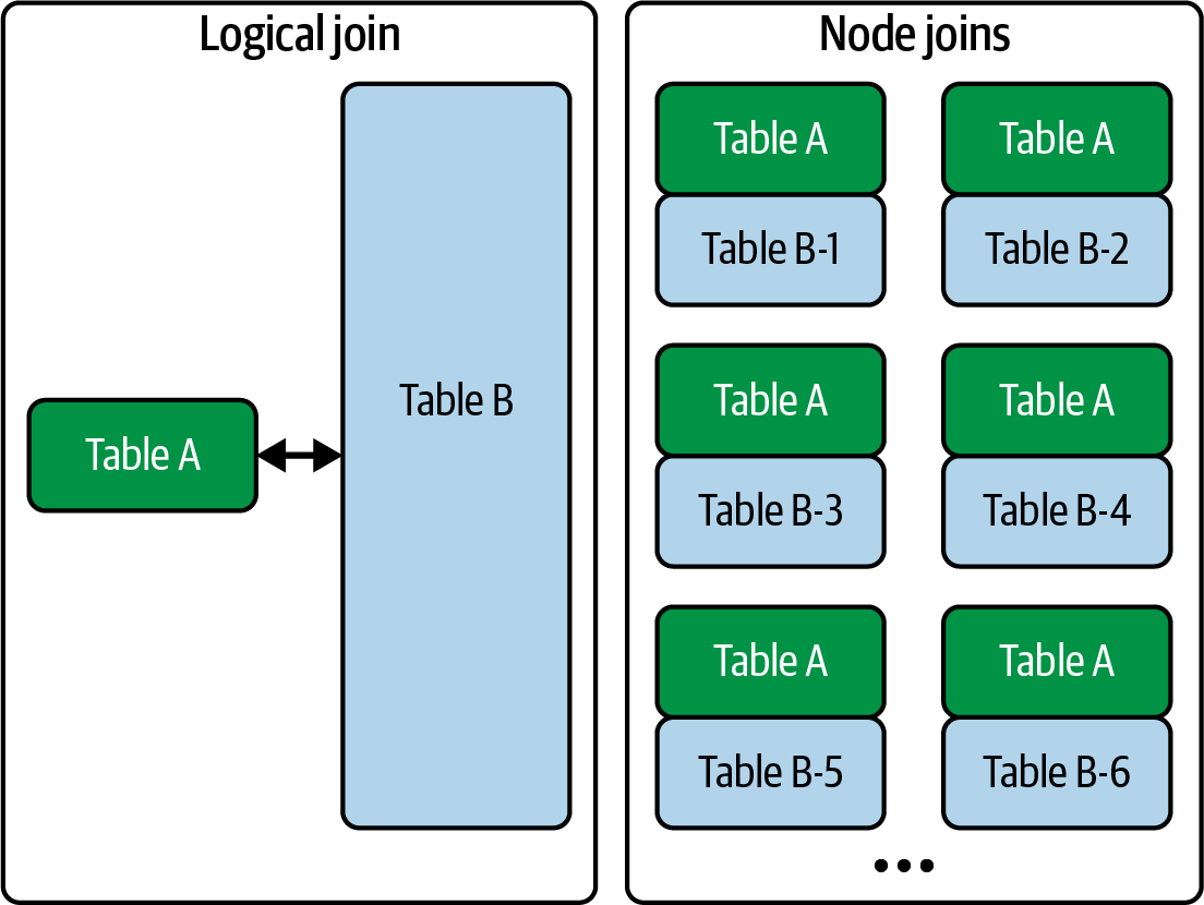 Figure 1. In a broadcast join, the query engine sends table A out to all nodes in the cluster to be joined with the various parts of table B
 -
A shuffle hash join is a symmetric distributed join where both large tables, incapable of fitting on a single node, are repartitioned and shuffled across the network by the join key using a hashing scheme, resulting in a more resource-intensive and less performant operation, often necessary when a broadcast join is not feasible.
A hashing scheme is a function that maps a data record’s join key to a specific node, ensuring all records with the same key are sent to that node for local joining. 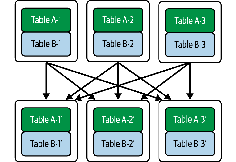 Figure 2. In a shuffle hash join, tables A and B are initially distributed across nodes, then repartitioned by a join key using a hashing scheme, reshuffled to specific nodes, and finally joined locally on those nodes.
7.3.1.2. ETL, ELT, and data pipelines
Traditional ETL (Extract, Transform, Load), a pattern driven by historical database limitations, typically used a dedicated external system to pull, transform, and clean data for a specific schema (like a Kimball star schema) before loading the final result into a data warehouse for business analytics.
In direct contrast, modern ELT (Extract, Load, Transform) reverses this pattern, leveraging the immense performance and storage of today’s data platforms (like warehouses, lakes, and lakehouses) to load raw data first and perform transformations using the platform’s own internal capabilities.
| Ingesting data without a plan is a great recipe for a data swamp. |
In current data architectures, the line between ETL and ELT is blurring, leading to the view that organizations should not standardize on one method but instead select the most appropriate technique for each individual data pipeline on a case-by-case basis.
7.3.1.3. SQL and Code-based Transformation Tools
SQL is a first-class citizen in big data ecosystems, and can be used to simplify data transformations with automatic optimization in SQL engines, whereas code-based tools like Spark offer more control but require manual optimization.
SQL is a declarative language to describe the desired data state, and despite its non-procedural nature, it can be used effectively to build complex data workflows and pipelines using common table expressions, scripts, or orchestration tools, sometimes more efficiently than procedural programming languages.
-
When determining whether to use SQL for batch transformations, consider avoiding it if the transformation is difficult, unreadable, or unmaintainable in SQL, or if reusable libraries are a necessity, as procedural languages are often better suited for such complex tasks.
-
Optimizing Spark and other code-heavy processing frameworks requires manual effort and adherence to best practices, including early filtering, reliance on core APIs, and careful UDF usage, contrasting with SQL’s automatic optimization.
7.3.1.4. Update patterns
Updating persisted data is a significant challenge in data engineering, particularly with evolving technologies, and the modern data lakehouse concept now integrates in-place updates, which are crucial for efficiency (avoiding full re-runs) and compliance with data deletion regulations like GDPR.
-
The truncate-and-reload update pattern is a method for refreshing data where the existing data in a table is completely erased and then replaced with a newly generated and transformed dataset.
-
The insert-only pattern is a method for maintaining a current data view by adding new, versioned records instead of altering existing ones, with the drawback of being slow when finding the latest record.
A materialized view speeds up queries on insert-only tables by acting as a truncate-and-reload target table that stores the pre-computed current state of the data. For a robust audit trail, the insert-only pattern treats data as a sequential, append-only log where new records are added but never changed. ✦ In column-oriented OLAP databases, single-row inserts are an anti-pattern that causes high system load and fragmented data storage, leading to inefficient reads; the recommended solution is to load data in batches or micro-batches.
✦ The enhanced Lambda architecture, found in systems like BigQuery and Druid, is an exception that handles frequent inserts by hybridizing a streaming buffer with columnar storage, although deletes and in-place updates can still be expensive.
In columnar databases, primary keys or uniqueness are not enforced by the system but are a logical construct that the data engineering team must manage with queries to define the current state of a table -
Deletion is a critical function for regulatory compliance but is a more expensive operation than an insert in columnar systems and data lakes.
A hard delete permanently removes a record from a database, while a soft delete marks the record as deleted.
-
Hard deletes are used to permanently remove data for performance, legal, or compliance reasons.
-
Soft deletes are used to filter records from query results without permanently deleting them.
The insert-only pattern can also be used to create a new record with a deletedflag instead of altering the original to enable soft deletes within an immutable, append-only framework.
-
-
The upsert and merge patterns are update strategies that match records against a target table using a key, where upsert will either insert a new record or update an existing one, while the merge pattern also adds the ability to delete records.
A merge operation is a superset of an upsert because, in addition to inserting and updating records, it also deletes records from the target table (the "old" data) that are absent from the source (the "new" data) with a full synchronization.
-
UPSERT=UPDATE+INSERT:-
If a record from the source matches a record in the target (based on a key), it UPDATEs the target record.
-
If a record from the source does not match any record in the target, it INSERTs the new record.
-
-
MERGE=UPDATE+INSERT+DELETE:-
It does everything an upsert does.
-
Additionally, if a record from the target table do not have a match in the source data, it DELETEs the target record.
-
Merging data in batches causes incorrect deletions because records outside the current batch are misinterpreted by the MERGE operation as not matched by source. A common solution is to use a staging table to first assemble the complete source dataset, which enables a single, reliable merge operation and avoids the issues of direct batch processing.
The pattern consists of the following steps:
-
First, a temporary staging table is completely cleared of any existing data, often with a
TRUNCATEcommand. -
Next, all batches of the source dataset are loaded into this staging table, typically using simple insert operations.
-
Finally, after the staging table holds the complete source dataset, a single
MERGEoperation is executed to synchronize the data from the staging table to the final target table.
The upsert and merge pattern was originally designed for row-based databases, where updates are a natural process that the database looks up the record in question and changes it in place. On the other hand, file-based systems don’t support in-place file updates, where the entire file must be rewritten even for single record changes, which led early big data and data lake adopters to reject updates in favor of insert-only patterns; however, columnar databases like Vertica have long supported in-place updates by abstracting the underlying Copy-on-Write complexity, a capability now common in major columnar cloud data warehouses. -
7.3.1.5. Schema updates
In modern cloud data warehouse, a new option for semi-structured data, borrowing from document stores, is typically used to provide flexibility for schema updates by storing frequently accessed data in flattened fields alongside raw JSON.
| Semi-structured data is a first-class citizen in data warehouses, opening new opportunities for data analysts and data scientists since data is no longer constrained to rows and columns. |
7.3.1.6. Data Wrangling
Data wrangling is the process of transforming messy, malformed data into useful, clean data, typically through a batch transformation process, and has historically been a challenging task for data engineers.
-
Data wrangling tools, often presented as no-code solutions or IDEs for malformed data, aim to automate and simplify the process of cleaning and transforming data, freeing data engineers for more complex tasks and enabling analysts to assist with parsing.
-
Graphical data-wrangling tools provide visual interfaces for analyzing data, defining processing steps to fix issues, and executing these on scalable systems like Spark with iterative refinement, making them highly recommended for streamlining engineering tasks and widely available.
7.3.1.7. Example: Data transformation in Spark
In a typical data pipeline, Airflow orchestrates the initial ingestion of JSON data from multiple APIs into an S3 bucket, then triggers a Spark job to process this data. The Spark job reads the raw files, transforms them into a unified relational table (i.e., dataframe), and filters the results with a SQL query. Finally, Spark writes the processed data back to S3 as a compressed, Parquet-formatted Delta Lake table, after which Airflow marks the entire workflow as complete.
7.3.1.8. MapReduce
MapReduce is a foundational batch data transformation pattern from the big data era, first introduced by Google and widely popularized as the original processing engine for Hadoop. Although it is not commonly used directly by data engineers today, its core principles continue to influence the design of modern distributed systems, and is still valuable for grasping the fundamentals of large-scale data processing.
The classic MapReduce model works in distinct stages: map, shuffle, and reduce. Initially, map tasks run in parallel across a cluster, with each task reading and processing an individual block of data. Afterwards, the shuffle phase redistributes the intermediate results, ensuring all data for a specific key is moved to a single node. Finally, the reduce step aggregates this grouped data on each node to compute the final result. A defining characteristic of this paradigm is its rigidity and reliance on disk, as all data is written to and read from disk between tasks, with no intermediate state held in memory.
Modern data processing has moved into a post-MapReduce world with frameworks like Spark and BigQuery that prioritize in-memory processing. These systems still employ the concepts of map, shuffle, and reduce but relax the older constraints by using RAM as the primary tier for holding data. Data is only spilled to disk when it exceeds available memory, which dramatically speeds up performance. The adoption of this faster, more flexible in-memory approach has been driven largely by the cloud, which makes it cost-effective to lease the necessary memory for the duration of a processing job.
7.3.2. Materialized Views, Federation, and Query Virtualization
-
A view is a stored query used to simplify data access or enhance security, while a materialized view is a stored result set, pre-computed and saved to improve performance.
-
A federated query is a database feature that allows an OLAP database to select from an external data source, such as object storage or RDBMS.
An external table is a database object that stores metadata about an external source (such as its location and file format) without ingesting the data itself, reading the data directly from that source only when the table is queried. -
Data virtualization is a practice where a query engine like Trino or Presto, which doesn’t store data internally, is used to directly query and access data scattered across various external systems.
-
A key feature called query pushdown optimizes performance by moving parts of a query to the source database, which leverages that system’s processing power and reduces network traffic.
-
Data virtualization is a good solution for organizations with data stored across various sources, however, it must be used carefully because directly querying a live production system can negatively impact its performance.
-
Data virtualization can also be used as a component in data ingestion pipelines to pull data from a production system during off-peak hours and save it to a data lake, which protects the source system from direct analytical queries.
A common strategy is to use it for scheduled data ingestion, pulling data during off-peak hours and saving it to a data lake. -
In a modern data mesh architecture, data virtualization can serve as a critical access layer that expands the data lake, providing a unified way for different teams to share their data products across the company.
-
8. Data Serving
Data serving is the final stage of the data engineering lifecycle, where prepared data is delivered for downstream use cases such as analytics and BI, machine learning applications, and reverse ETL.
When serving data, several key factors must be considered to ensure it is effective and valuable. The most crucial consideration is trust; end-users must have confidence in the data’s quality, accuracy, and reliability, which is built and maintained through data validation, observability, and upholding Service Level Agreements (SLAs).
It is also vital to understand the use case and the user. Data should be action-oriented, and engineers should prioritize projects with the highest return on investment by understanding who will use the data and for what purpose. This leads to treating data as a data product, which involves understanding the user’s "job to be done" and creating solutions that meet their specific needs. A good data product is the result of understanding its users' goals, its specific audience (internal or external), and its expected return on investment, which in turn drives adoption and continuous improvement and feedback.
While the concept of self-service data is a popular aspiration, it is difficult to implement successfully and often fails in practice. The primary reason for failure is a mismatch between the self-service tools and the end-users' actual needs, as executives typically prefer pre-built, actionable dashboards while analysts already use more powerful tools like SQL.
Furthermore, data definitions and logic must be formally defined, documented, and consistently applied to ensure correctness, which prevents reliance on ambiguous institutional knowledge and can be managed effectively through a semantic layer. A data definition provides the specific, agreed-upon meaning of a term, such as what qualifies as a "customer," across all departments. Data logic, in turn, consists of the formal rules and formulas that use these definitions to derive key metrics, like "customer lifetime value."
Finally, an emerging consideration is the data mesh, an organizational structure that decentralizes data serving. In this model, domain-specific teams are responsible for both producing and consuming data, treating it as a product to be shared across the organization.
| In the serving stage, data engineers interface with a wide range of stakeholders, including data analysts, data scientists, ML engineers, and business users, where the primary responsibility is to provide the highest-quality data products possible, not to interpret the data’s end uses. This support role requires managing feedback loops as data is rarely static, and establishing a clear separation of duties is crucial as a company matures to avoid unsustainable role overlap. In a data mesh architecture, these responsibilities are decentralized, requiring domain teams to effectively collaborate and manage their own data serving tasks. |
8.1. Analytics
Analytics is a data-serving use case for discovering key insights, where success depends on first identifying the end goal to determine the right type of analytics to apply—such as business analytics for historical trends, operational analytics for real-time alerts, or embedded analytics for in-app dashboards.
8.1.1. Business analytics
Business analytics is the practice of using historical and current data to inform strategic, actionable decisions by combining statistical and trend analysis with domain expertise and human judgment. It is considered both an art and a science, primarily manifesting in dashboards, reports, and ad hoc analysis.
-
A dashboard is a business intelligence tool that provides a concise, visual summary of an organization’s performance against its most critical metrics, much like a car’s dashboard displays essential information for a driver. Tailored for decision-makers, dashboards can range from high-level executive overviews to more detailed views for specific departments, tracking KPIs and OKRs. Analysts are responsible for creating, maintaining, and updating these dashboards using BI platforms such as Tableau, Looker, or Power BI.
-
A report is a detailed analysis created to answer a specific business question, with the goal of using data to drive insights and action. Unlike a dashboard’s ongoing monitoring, a report is typically a one-time investigation into a particular issue, such as an analyst querying a data warehouse to determine the root cause of high product returns. The findings are then summarized and distributed to relevant stakeholders, often using the same BI tool where dashboards are hosted.
-
Ad hoc analysis is a one-time, exploratory investigation into a specific business question or issue, often serving as the starting point for what may later become a formal report or a new metric on a dashboard if the insights are significant. The tools for ad hoc analysis overlap with those for reports and dashboards but also frequently include more flexible options like Excel, Python or R notebooks, and direct SQL queries.
| BI systems share the data processing workload with a source database, but the approach varies, like Tableau, pull data from the database to store and process it locally for interactive analysis. In contrast, modern BI systems like Looker use a query pushdown model, where they translate user interactions and predefined logic into SQL queries that are executed directly on the source database. To improve performance, both types of systems commonly use caching for frequently run queries. |
A collaborative relationship between analysts and data engineers is crucial for effective business analytics; analysts provide vital feedback on data quality and request new datasets, while engineers are responsible for ingesting and preparing this data. This partnership creates a virtuous cycle, as demonstrated when engineers ingest supply-chain data that allows analysts to pinpoint a faulty supplier, leading to a direct business impact.
Data for analytics is typically served in batches from a data warehouse or lake at widely varying frequencies, but it is critical to remember that the initial ingestion frequency sets the speed limit for all downstream processes. Therefore, even if current use cases are batch-oriented, data from a streaming source should be ingested as a stream to preserve future real-time capabilities.
Finally, data engineers must consider the backend architecture, as some BI tools use an internal storage layer while others query the data warehouse directly. The direct-query approach leverages the power of the underlying database but requires careful management of cost, access control, and latency.
8.1.2. Operational Analytics
Operational analytics is distinguished from business analytics by its focus on using real-time data to take immediate action, whereas business analytics uses data to derive longer-term actionable insights. The key difference is the element of time; operational analytics requires up-to-the-second data to address problems as they happen.
| The distinction between the two is blurring as streaming data becomes more common, pushing data products toward a streaming-first future. This trend underscores the principle that the value of real-time data is contingent on taking correct action, without which it is merely a distraction. |
Real-time application monitoring is a primary example of operational analytics, enabling software engineering teams to track key performance metrics like requests per second or database I/O on a live dashboard, which allows for immediate, automated actions, such as triggering server scaling events when load increases or sending alerts via text, chat, or email when critical thresholds are breached.
8.1.3. Embedded Analytics
Embedded analytics are external-facing dashboards and metrics integrated directly into an application for the end user that, in contrast to the internal focused business and operational analytics, provide users with data about their own interactions to empower better, often real-time, decisions.
For instance, a smart thermostat app empowers users by showing real-time power consumption to help them create more energy-efficient schedules, while an e-commerce platform might provide sellers with a live dashboard of sales and inventory to inform timely customer deals. In both cases, the application uses embedded analytics to provide data that allows the end user to make immediate, data-driven decisions.
| Data engineers supporting embedded analytics must provide backend databases that solve three key performance challenges: low data latency, fast query performance, and high concurrency. |
8.2. Machine Learning
Machine learning (ML), a field of artificial intelligence where computer systems learn from data to make predictions and decisions, relies on a collaborative data serving process where data engineers prepare and deliver tailored data for model training and execution, involving transforming raw data into numerical features through featurization, such as encoding categorical data and creating embeddings, and implementing and maintaining robust data pipelines for both batch and streaming delivery to feed ML models, often in collaboration with ML engineers.
While a data engineer doesn’t need to have a deep understanding of ML, a foundational knowledge of its core principles is essential for effectively supporting the machine learning lifecycle. This includes understanding fundamental concepts such as the differences between supervised and unsupervised learning, classification, and regression, and knowing when to use classical algorithms versus deep learning. Proficiency in data-centric tasks like data wrangling, feature engineering, and handling time-series data is also crucial. Furthermore, a data engineer should grasp the operational aspects of ML, such as the distinctions between batch and online learning, the implications of different hardware choices (CPU vs. GPU), the role of technologies like feature stores, and the importance of data quality to prevent issues like data cascades.
9. Data Serving for Analytics and ML
Data engineers empower analytics and machine learning by serving data through a comprehensive suite of methods, including traditional file exchanges and databases, modern streaming and federated query systems, as well as advanced options like data sharing platforms, semantic layers, and direct notebook integration.
9.1. File Exchange
File exchange is a common method for serving structured, semi-structured, and unstructured data to consumers. The way files are served depends on factors like the use case, the consumer’s data handling processes, file size, and data type. Simple methods like emailing files are problematic due to a lack of version control and access revocation, making collaboration platforms like Google Docs or Microsoft 365 preferable for maintaining a single, consistent version of a file. For larger-scale needs, file exchange evolves into using object storage or data lakes. However, at that scale, it is often considered a more streamlined process akin to data sharing rather than a simple ad-hoc file exchange.
9.2. Databases
Databases, particularly OLAP systems like data warehouses and data lakes, are a critical layer for serving data in analytics and ML. The process involves querying the database and consuming the results, for instance by exporting them to a CSV file or analyzing them in a notebook. Serving data from a database offers significant benefits, including the order and structure imposed by schemas, the ability to implement fine-grained access controls at the table, column, and row levels, and high performance for computationally intensive queries and high concurrency. For example, in a machine learning workflow, a data scientist might connect to a database to extract data, perform feature engineering and selection, and then feed the resulting dataset into an offline model for training and generating predictions.
9.3. Streaming Systems
Streaming systems are increasingly vital for serving data in analytics and ML, representing a paradigm shift from traditional queries to continuously emitted metrics. A key development in this area is the rise of operational analytics databases, which combine the features of OLAP databases and stream-processing systems, which allows queries to run on a vast range of data, from historical to the most current, up-to-the-second information.
9.4. Query Federation
Query federation is a pattern that allows a single query to pull data from multiple diverse sources—like data lakes, databases, and data warehouses—without first centralizing the data. This approach offers significant flexibility for ad-hoc exploratory analysis and is ideal for situations where data access needs to be tightly controlled, providing secure, read-only access that is beneficial for compliance.
However, this method presents challenges, primarily the risk of federated queries consuming excessive resources on live production systems. It serves as a practical way to blend data and determine if the performance is sufficient for ongoing needs or if a more permanent solution, like centralizing the data into an OLAP system via ETL pipelines, is required.
9.5. Data Sharing
Data sharing is a serving model where data is exchanged between different organizations or business units through massively multitenant cloud storage systems like Snowflake, Redshift, and BigQuery. In this pattern, the responsibility for running queries shifts from the data engineers to the data consumers (analysts and data scientists). This reframes the primary challenge of data serving into one of managing security and access control, making it a compelling and increasingly core feature of major data platforms for sharing data safely and securely.
9.6. Semantic and Metrics Layers
A semantic or metrics layer is a tool that standardizes business logic to ensure that queries produce accurate and consistent analytics, built on the principle that even the most powerful query engines will quickly return bad results when fed poor-quality queries.
These layers solve this problem by providing a central place to define and maintain key business metrics. Tools like Looker (with LookML) or dbt (Data Build Tool) allow for the creation of reusable, complex business logic. When a user requests a metric, the tool generates the correct SQL query based on this standardized definition, which prevents the inconsistencies and repetition found in traditional ETL scripts.
-
Looker, using its language LookML, operates primarily at the serving and reporting layer. It defines business logic virtually and generates complex SQL queries on the fly when a user interacts with a report or dashboard.
-
dbt, in contrast, operates exclusively in the transformation layer. It serves as a robust pipeline orchestration tool for analytics engineers to build and materialize data models directly in the warehouse, which BI tools then query.
By ensuring that everyone in an organization uses the same underlying calculations for the same business concepts, these tools directly address the critical question, "Are these numbers correct?" and build trust in the data.
9.7. Notebooks
Serving data to notebooks, the primary tool for data scientists, begins with establishing programmatic connections to sources like databases, data lakes, or APIs. A key role for the data engineer is to assist data scientists in discovering the correct data and ensuring they have the proper permissions to access it.
A common workflow for data scientists is to load data into a pandas DataFrame on a local machine, which inevitably fails when the dataset’s size exceeds the available memory. The solution is to guide data scientists off their laptops and onto scalable cloud infrastructure. This transition typically follows a path from cloud-hosted notebooks to distributed execution systems (like Dask, Ray, or Spark) and eventually to fully managed ML platforms such as SageMaker, Vertex AI, or Azure ML. Data and ML engineers are crucial in leading this move by setting up the infrastructure, managing environments, and training scientists on these more powerful tools.
Finally, notebooks can even be used in production to accelerate deployment, an approach with significant trade-offs. While it allows data scientists to move faster, it is often considered a substandard production practice. The alternative, having engineers rewrite notebooks for production, creates a bottleneck. A hybrid approach is often ideal, where notebooks are used for light production tasks and a full, robust productionization process is reserved for high-value projects.
10. Reverse ETL
Reverse ETL is the process of serving data by taking processed information from an analytical system, like a data warehouse, and loading it back into an operational source system, such as a CRM or marketing platform. The primary goal is to reduce friction for end-users by delivering valuable data directly into the tools they use for their daily work. For example, instead of providing a sales team with a separate dashboard, reverse ETL would load machine learning-generated lead scores directly into the customer profiles within their CRM.
While the name "reverse ETL" is not perfectly descriptive, the practice of moving data from OLAP systems back into source systems is an increasingly important and formalized data engineering responsibility. Although custom solutions can be built, it is often better to use one of the many available open-source or commercial tools, keeping in mind that the vendor landscape is new and changing rapidly.
A significant word of caution is that reverse ETL inherently creates feedback loops. If an error exists in the processing logic (e.g., an ad bidding model), feeding the flawed output back into the source system can amplify the error, potentially leading to major negative consequences like wasting massive amounts of money. Therefore, it is critical to implement robust monitoring and guardrails when using this serving pattern.
Appendix A: Serialization and Compression
A.1. Serialization Formats
Serialization, the process of converting data for storage or transmission, is a critical foundation of data engineering where the choice of format has massive performance implications. The primary decision lies between row-oriented formats (like JSON and Avro), which excel at handling individual records, and columnar formats (like Parquet), which are highly optimized for large-scale analytical queries through efficient I/O and compression.
Modern innovations are advancing the field even further. Apache Arrow provides a standard for in-memory columnar data to eliminate serialization overhead between processes, while hybrid table formats like Apache Iceberg and Hudi act as a management layer on top of these formats to provide reliable, transactional capabilities and features like time travel directly on the data lake.
A.1.1. Row-Based Serialization
Row-based serialization formats, such as the archetypal CSV, organize data by row. For semistructured data (data objects that support nesting and schema variation), row-oriented serialization entails storing each object as a unit.
-
CSV is a slow and error-prone "nonstandard standard" due to its many variations in conventions, such as different delimiters and quoting rules, which makes it unsuitable for data pipelines. When using CSV exchanging data with external systems or for data archival, it is critical to provide a complete technical description of the specific format configuration to ensure the data remains usable in the future.
-
Extensible Markup Language (XML) is a legacy format that is generally slow to serialize and deserialize in data engineering applications. Although largely replaced by JSON for plain-text object serialization, data engineers are still often required to use XML when interacting with legacy systems.
-
JavaScript Object Notation (JSON) has become the modern standard for data exchange over APIs and is a popular format for data storage. Its widespread native support in major databases, from document stores to cloud data warehouses, simplifies the process of moving data between applications and analytical systems.
-
JSONL (JSON Lines) is a specialized format that stores bulk semistructured data by delimiting each JSON object with a line break, making it highly effective for initial data ingestion. For subsequent pipeline stages, however, JSONL should be converted into a more performant columnar format to optimize for transformation and serving.
-
Avro is a row-oriented data format designed for RPCs and data serialization, which encodes data into a compact binary format while defining the schema separately in JSON. It is a popular format within the Hadoop ecosystem and is also supported by many cloud data tools.
A.1.2. Columnar Serialization
Columnar serialization organizes data by storing each column in its own set of files, a fundamental pivot from row-oriented formats, which is highly optimized for analytical workloads because queries need to scan only the necessary columns instead of entire rows, and grouping similar data together enables highly efficient compression, such as tokenization for repeated values and standard algorithms for redundant data, which maximizes storage and network resources.
| Columnar formats are inefficient for record-level operations because accessing a single record requires reconstruction from multiple files, and updating a field is extremely costly due to the need to decompress and rewrite entire column segments, which makes them ill-suited for transactional (OLTP) workloads that rely on more efficient row-oriented storage. |
-
Parquet is a columnar format designed for high performance in data lakes. It improves on formats like CSV by including schema information and native support for nested data. Crucially, Parquet is also highly portable, avoiding the significant performance penalties that proprietary warehouse formats incur when used with external data lake tools like Spark. To maximize efficiency, Parquet is almost always used with a compression codec, such as the speed-optimized Snappy algorithm.
-
Optimized Row Columnar (ORC) is a columnar storage format similar to Parquet, which was historically popular for its use with Apache Hive. Although still widely used, ORC is now generally less common than Parquet and has more limited support across the modern cloud data ecosystem. This support gap is illustrated by tools like Snowflake and BigQuery, which can import data from ORC files but, unlike with Parquet, cannot export data back into the ORC format.
-
Apache Arrow is an in-memory, language-agnostic columnar format designed to eliminate the significant performance overhead of traditional serialization and deserialization. It achieves this by providing a single, standardized binary format that can be used for high-performance data processing in memory, transfer over the network, and long-term storage, thus avoiding costly data conversion steps.
To address the challenge of different programming languages having unique memory layouts, the Arrow project provides libraries that allow diverse languages like Java, Python, and C++ to work on the same data in memory with zero-copy efficiency. This powerful interoperability has led to its rapid adoption in major frameworks like Apache Spark and has inspired new, Arrow-native data platforms such as Dremio.
A.1.3. Hybrid Serialization
Hybrid serialization refers to technologies, such as Apache Hudi and Apache Iceberg, that either combine multiple serialization techniques or integrate a serialization format with an additional abstraction layer for tasks like schema management.
-
Apache Hudi (Hadoop Update Delete Incremental) is a table management technology that enables both high-performance analytical queries and atomic, transactional updates on the same table. It achieves this with a hybrid approach, storing the bulk of the data in a columnar format for fast analytics while ingesting new updates from streams (like CDC) into a row-oriented format for write efficiency. Queries provide a real-time view by combining data from both formats, and a periodic repacking process merges the row-based updates into the columnar store to maintain long-term query performance.
-
Like Hudi, Apache Iceberg is a table management technology that tracks the individual files making up a data lake table, and through this snapshot-tracking ability, it enables key features such as table time travel (the ability to query the table as it existed at a specific point in the past), robust schema evolution, and the management of petabyte-scale tables.
A.2. Compression
Compression algorithms reduce data size by identifying and removing redundancy and repetition, then re-encoding the data into a more compact format. The process is reversed during decompression to perfectly reconstruct the original data. A simple analogy is replacing frequently used words in a text with shorter tokens; sophisticated algorithms use advanced mathematical techniques to achieve much higher compression ratios, often reaching 10:1 for text.
Lossless compression restores a bit-for-bit exact copy of the original data upon decompression, which is critical for analytics where data fidelity must be perfect. In contrast, lossy compression, used for audio, images, and video, recovers a version that looks or sounds like the original but is not an exact copy, as it prioritizes reducing file size over perfect data integrity.
Traditional compression algorithms like gzip and bzip2 excel at achieving high compression ratios, especially for text-based formats such as JSON and CSV. In contrast, a newer generation of algorithms, including Snappy, Zstandard, and LZ4, prioritizes high-speed performance and CPU efficiency over achieving the maximum possible compression. These faster algorithms are commonly used in data lakes and columnar databases where quick query performance is more critical than minimizing storage size.
|
|
|
A |
The effectiveness of compression hinges on the data’s redundancy, making text-based data such as logs, JSON, and CSV files excellent targets due to their highly repetitive nature. Similarly, raw uncompressed binary formats like bitmap images are also good candidates. However, it is inefficient to compress data that is already in a compressed format, as this provides little to no additional size reduction. This category of poor targets includes common media files like JPEG and MP3, archive files like ZIP, and application packages like JAR and DLL files, all of which contain internal compression or have low redundancy, making them unsuitable for further compression.
Streaming compression works by breaking the continuous data flow into manageable chunks or blocks, as the entire stream is not available at once. To effectively find patterns, algorithms use a sliding window that maintains a buffer of the most recent data to use as a dictionary for compressing the current chunk. Each compressed chunk is then wrapped in a self-contained frame that includes metadata, such as its size and a checksum. This creates a continuous stream of independent frames, allowing a decompressor on the receiving end to read and decompress each piece individually to reconstruct the original data flow.