Alex Petrov - Database Internals

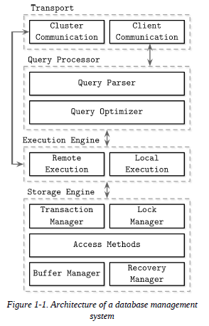
Databases are modular systems and consist of multiple parts: a transport layer accepting requests, a query processor determining the most efficient way to run queries, an execution engine carrying out the operations, and a storage engine.

The storage engine (or database engine) is a software component of a database management system responsible for storing, retrieving, and managing data in memory and on disk, designed to capture a persistent, long term memory of each node. While databases can respond to complex queries, storage engines look at the data more granularly and offer a simple data manipulation API, allowing users to create, update, delete, and retrieve records. One way to look at this is that database management systems are applications built on top of storage engines, offering a schema, a query language, indexing, transactions, and many other useful features.

The more knowledge you have about the database before using it, the more time you’ll save when running it in production.

Online transaction processing (OLTP) databases

• These handle a large number of user-facing requests and transactions.

• Queries are often predefined and short-lived.

Online analytical processing (OLAP) databases

• These handle complex aggregations.

• OLAP databases are often used for analytics and data warehousing, and are capable of handling complex, long-running ad hoc queries.

Hybrid transactional and analytical processing (HTAP)

• These databases combine properties of both OLTP and OLAP stores.

DBMS Architecture

Column- Versus Row-Oriented DBMS

Most database systems store a set of data records, consisting of columns and rows in tables. Field is an intersection of a column and a row: a single value of some type. Fields belonging to the same column usually have the same data type. A collection of values that belong logically to the same record (usually identified by the key) constitutes a row.

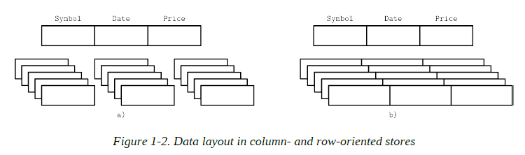
One of the ways to classify databases is by how the data is stored on disk: row- or column-wise. Tables can be partitioned either horizontally (storing values belonging to the same row together), or vertically (storing values belonging to the same column together).

Row-Oriented Data Layout

Row-oriented database management systems store data in records or rows. Their layout is quite close to the tabular data representation, where every row has the same set of fields.

| ID | Name | Birth Date | Phone Number |
| 10 | John | 01 Aug 1981 | +1 111 222 333 |
| 20 | Sam | 14 Sep 1988 | +1 555 888 999 |
| 30 | Keith | 07 Jan 1984 | +1 333 444 555 |

This approach works well for cases where several fields constitute the record (name, birth date, and a phone number) uniquely identified by the key (in this example, a monotonically incremented number). All fields representing a single user record are often read together. When creating records (for example, when the user fills out a registration form), we write them together as well. At the same time, each field can be modified individually.

Since row-oriented stores are most useful in scenarios when we have to access data by row, storing entire rows together improves spatial locality.

Because data on a persistent medium such as a disk is typically accessed block-wise (in other words, a minimal unit of disk access is a block), a single block will contain data for all columns. This is great for cases when we’d like to access an entire user record, but makes queries accessing individual fields of multiple user records (for example, queries fetching only the phone numbers) more expensive, since data for the other fields will be paged in as well.

Column-Oriented Data Layout

Column-oriented database management systems partition data vertically (i.e., by column) instead of storing it in rows. Here, values for the same column are stored contiguously on disk (as opposed to storing rows contiguously as in the previous example).

Storing values for different columns in separate files or file segments allows efficient queries by column, since they can be read in one pass rather than consuming entire rows and discarding data for columns that weren’t queried.

Column-oriented stores are a good fit for analytical workloads that compute aggregates, such as finding trends, computing average values, etc.

From a logical perspective, the data representing stock market price quotes can still be expressed as a table:

| ID | Symbol | Date | Price |
| 1 | DOW | 08 Aug 2018 | 24,314.65 |
| 2 | DOW | 09 Aug 2018 | 24,136.16 |
| 3 | S&P | 08 Aug 2018 | 2,414.45 |
| 4 | S&P | 09 Aug 2018 | 2,232.32 |

However, the physical column-based database layout looks entirely different. Values belonging to the same row are stored closely together:

Symbol: 1:DOW; 2:DOW; 3:S&P; 4:S&P
Date:   1:08 Aug 2018; 2:09 Aug 2018; 3:08 Aug 2018; 4:09 Aug 2018
Price:  1:24,314.65; 2:24,136.16; 3:2,414.45; 4:2,232.32

To reconstruct data tuples, which might be useful for joins, filtering, and multirow aggregates, we need to preserve some metadata on the column level to identify which data points from other columns it is associated with. If you do this explicitly, each value will have to hold a key, which introduces duplication and increases the amount of stored data. Some column stores use implicit identifiers (virtual IDs) instead and use the position of the value (in other words, its offset) to map it back to the related values.

Distinctions and Optimizations

It is not sufficient to say that distinctions between row and column stores are only in the way the data is stored. Choosing the data layout is just one of the steps in a series of possible optimizations that columnar stores are targeting.

Reading multiple values for the same column in one run significantly improves cache utilization and computational efficiency. On modern CPUs, vectorized instructions can be used to process multiple data points with a single CPU instruction (SIMD).

Storing values that have the same data type together (e.g., numbers with other numbers, strings with other strings) offers a better compression ratio. We can use different compression algorithms depending on the data type and pick the most effective compression method for each case.

To decide whether to use a column- or a row-oriented store, you need to understand your access patterns. If the read data is consumed in records (i.e., most or all of the columns are requested) and the workload consists mostly of point queries and range scans, the row-oriented approach is likely to yield better results. If scans span many rows, or compute aggregate over a subset of columns, it is worth considering a column-oriented approach.

Wide Column Stores

Column-oriented databases should not be mixed up with wide column stores, such as BigTable or HBase, where data is represented as a multidimensional map, columns are grouped into column families (usually storing data of the same type), and inside each column family, data is stored row-wise.

Data Files and Index Files

The primary goal of a database system is to store data and to allow quick access to it.

Database systems do use files for storing the data, but instead of relying on filesystem hierarchies of directories and files for locating records, they compose files using implementation-specific formats.

Database systems store data records, consisting of multiple fields, in tables, where each table is usually represented as a separate file. Each record in the table can be looked up using a search key. To locate a record, database systems use indexes: auxiliary data structures that allow it to efficiently locate data records without scanning an entire table on every access. Indexes are built using a subset of fields identifying the record.

A database system usually separates data files and index files: data files store data records, while index files store record metadata and use it to locate records in data files. Index files are typically smaller than the data files. Files are partitioned into pages, which typically have the size of a single or multiple disk blocks. Pages can be organized as sequences of records or as a slotted pages.

New records (insertions) and updates to the existing records are represented by key/value pairs. Most modern storage systems do not delete data from pages explicitly. Instead, they use deletion markers (also called tombstones), which contain deletion metadata, such as a key and a timestamp. Space occupied by the records shadowed by their updates or deletion markers is reclaimed during garbage collection, which reads the pages, writes the live (i.e., nonshadowed) records to the new place, and discards the shadowed ones.

Data Files

Data files (sometimes called primary files) can be implemented as index-organized tables (IOT), heap-organized tables (heap files), or hash-organized tables (hashed files).

Records in heap files are not required to follow any particular order, and most of the time they are placed in a write order. This way, no additional work or file reorganization is required when new pages are appended. Heap files require additional index structures, pointing to the locations where data records are stored, to make them searchable.

In hashed files, records are stored in buckets, and the hash value of the key determines which bucket a record belongs to. Records in the bucket can be stored in append order or sorted by key to improve lookup speed.

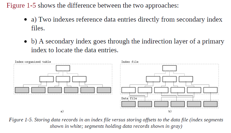
Index-organized tables (IOTs) store data records in the index itself. Since records are stored in key order, range scans in IOTs can be implemented by sequentially scanning its contents.

Storing data records in the index allows us to reduce the number of disk seeks by at least one, since after traversing the index and locating the searched key, we do not have to address a separate file to find the associated data record.

When records are stored in a separate file, index files hold data entries, uniquely identifying data records and containing enough information to locate them in the data file. For example, we can store file offsets (sometimes called row locators), locations of data records in the data file, or bucket IDs in the case of hash files. In index-organized tables, data entries hold actual data records.

Index Files

An index is a structure that organizes data records on disk in a way that facilitates efficient retrieval operations. Index files are organized as specialized structures that map keys to locations in data files where the records identified by these keys (in the case of heap files) or primary keys (in the case of index-organized tables) are stored.

An index on a primary (data) file is called the primary index. However, in most cases we can also assume that the primary index is built over a primary key or a set of keys identified as primary. All other indexes are called secondary.

Secondary indexes can point directly to the data record, or simply store its primary key. A pointer to a data record can hold an offset to a heap file or an index-organized table. Multiple secondary indexes can point to the same record, allowing a single data record to be identified by different fields and located through different indexes. While primary index files hold a unique entry per search key, secondary indexes may hold several entries per search key.

If the order of data records follows the search key order, this index is called clustered (also known as clustering). Data records in the clustered case are usually stored in the same file or in a clustered file, where the key order is preserved. If the data is stored in a separate file, and its order does not follow the key order, the index is called nonclustered (sometimes called unclustered).

NOTE: Index-organized tables store information in index order and are clustered by definition. Primary indexes are most often clustered. Secondary indexes are nonclustered by definition, since they’re used to facilitate access by keys other than the primary one. Clustered indexes can be both index-organized or have separate index and data files.

Primary Index as an Indirection

By referencing data directly, we can reduce the number of disk seeks, but have to pay a cost of updating the pointers whenever the record is updated or relocated during a maintenance process. Using indirection in the form of a primary index allows us to reduce the cost of pointer updates, but has a higher cost on a read path.

Updating just a couple of indexes might work if the workload mostly consists of reads, but this approach does not work well for write-heavy workloads with multiple indexes. To reduce the costs of pointer updates, instead of payload offsets, some implementations use primary keys for indirection.

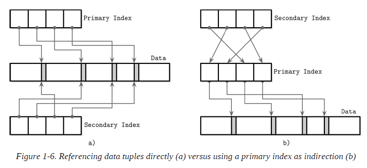
It is also possible to use a hybrid approach and store both data file offsets and primary keys. First, you check if the data offset is still valid and pay the extra cost of going through the primary key index if it has changed, updating the index file after finding a new offset.

Buffering, Immutability, and Ordering

Storage structures have three common variables: they use buffering (or avoid using it), use immutable (or mutable) files, and store values in order (or out of order). Most of the distinctions and optimizations in storage structures discussed are related to one of these three concepts.

Buffering

This defines whether or not the storage structure chooses to collect a certain amount of data in memory before putting it on disk. Of course, every on-disk structure has to use buffering to some degree, since the smallest unit of data transfer to and from the disk is a block, and it is desirable to write full blocks.

Mutability (or immutability)

This defines whether or not the storage structure reads parts of the file, updates them, and writes the updated results at the same location in the file. Immutable structures are append-only: once written, file contents are not modified. Instead, modifications are appended to the end of the file. There are other ways to implement immutability. One of them is copy-on-write , where the modified page, holding the updated version of the record, is written to the new location in the file, instead of its original location. Often the distinction between LSM and B-Trees is drawn as immutable against in-place update storage, but there are structures (for example, Bw-Trees) that are inspired by B-Trees but are immutable.

Ordering

This is defined as whether or not the data records are stored in the key order in the pages on disk. In other words, the keys that sort closely are stored in contiguous segments on disk. Ordering often defines whether or not we can efficiently scan the range of records, not only locate the individual data records. Storing data out of order (most often, in insertion order) opens up for some write-time optimizations.

One of the most popular storage structures is a B-Tree. Many open source database systems are B-Tree based, and over the years they’ve proven to cover the majority of use cases.

Binary Search Trees

A binary search tree (BST) is a sorted in-memory data structure, used for efficient key-value lookups. BSTs consist of multiple nodes. Each tree node is represented by a key, a value associated with this key, and two child pointers (hence the name binary). BSTs start from a single node, called a root node. There can be only one root in the tree.

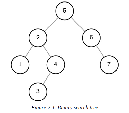
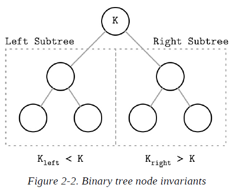
Each node splits the search space into left and right subtrees, a node key is greater than any key stored in its left subtree and less than any key stored in its right subtree

Following left pointers from the root of the tree down to the leaf level (the level where nodes have no children) locates the node holding the smallest key within the tree and a value associated with it. Similarly, following right pointers locates the node holding the largest key within the tree and a value associated with it. Values are allowed to be stored in all nodes in the tree. Searches start from the root node, and may terminate before reaching the bottom level of the tree if the searched key was found on a higher level.

Tree Balancing

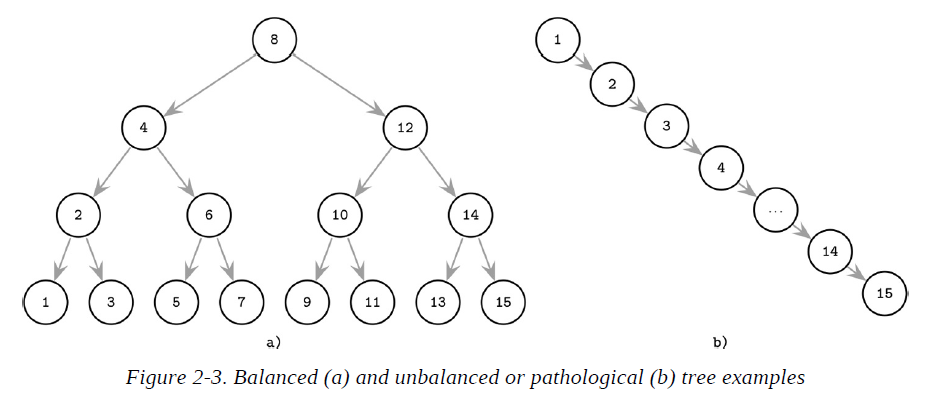
The balanced tree is defined as one that has a height of log2N, where N is the total number of items in the tree, and the difference in height between the two subtrees is not greater than one.

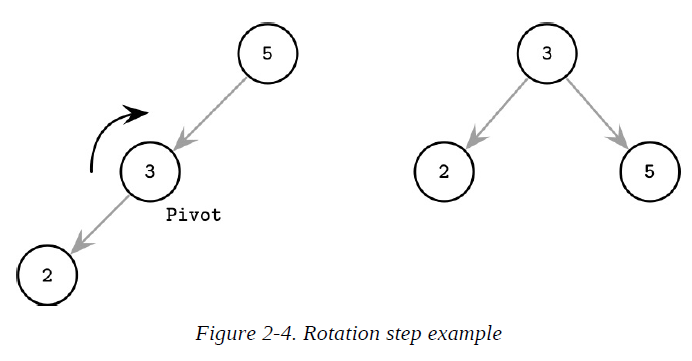
One of the ways to keep the tree balanced is to perform a rotation step after nodes are added or removed. If the insert operation leaves a branch unbalanced (two consecutive nodes in the branch have only one child), we can rotate nodes around the middle one.

Trees for Disk-Based Storage

BST, due to low fanout (fanout is the maximum allowed number of children per node), we have to perform balancing, relocate nodes, and update pointers rather frequently. Increased maintenance costs make BSTs impractical as on-disk data structures.

If we wanted to maintain a BST on disk, we’d face several problems.

• One problem is locality: since elements are added in random order, there’s no guarantee that a newly created node is written close to its parent, which means that node child pointers may span across several disk pages.

• Another problem, closely related to the cost of following child pointers, is tree height. Since binary trees have a fanout of just two, height is a binary logarithm of the number of the elements in the tree, and we have to perform O(log2N) seeks to locate the searched element and, subsequently, perform the same number of disk transfers. 2-3-Trees and other low-fanout trees have a similar limitation: while they are useful as in-memory data structures, small node size makes them impractical for external storage.

• A naive on-disk BST implementation would require as many disk seeks as comparisons, since there’s no built-in concept of locality.

Fanout and height are inversely correlated: the higher the fanout, the lower the height. If fanout is high, each node can hold more children, reducing the number of nodes and, subsequently, reducing height.

On-disk data structures are often used when the amounts of data are so large that keeping an entire dataset in memory is impossible or not feasible. Only a fraction of the data can be cached in memory at any time, and the rest has to be stored on disk in a manner that allows efficiently accessing it.

Hard Disk Drives

On spinning disks, seeks increase costs of random reads because they require disk rotation and mechanical head movements to position the read/write head to the desired location. However, once the expensive part is done, reading or writing contiguous bytes (i.e., sequential operations) is relatively cheap.

The smallest transfer unit of a spinning drive is a sector, so when some operation is performed, at least an entire sector can be read or written. Sector sizes typically range from 512 bytes to 4 Kb.

Head positioning is the most expensive part of an operation on the HDD. This is one of the reasons we often hear about the positive effects of sequential I/O: reading and writing contiguous memory segments from disk.

Solid State Drives

Solid state drives (SSDs) do not have moving parts: there’s no disk that spins, or head that has to be positioned for the read. A typical SSD is built of memory cells, connected into strings (typically 32 to 64 cells per string), strings are combined into arrays, arrays are combined into pages, and pages are combined into blocks.

Depending on the exact technology used, a cell can hold one or multiple bits of data. Pages vary in size between devices, but typically their sizes range from 2 to 16 Kb. Blocks typically contain 64 to 512 pages. Blocks are organized into planes and, finally, planes are placed on a die. SSDs can have one or more dies.

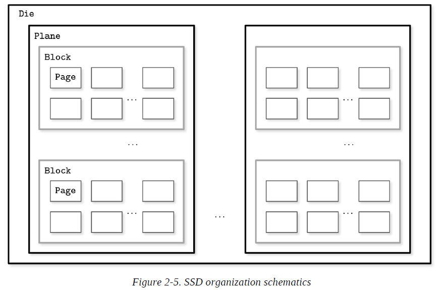
The smallest unit that can be written (programmed) or read is a page. However, we can only make changes to the empty memory cells (i.e., to ones that have been erased before the write). The smallest erase entity is not a page, but a block that holds multiple pages, which is why it is often called an erase block. Pages in an empty block have to be written sequentially.

The part of a flash memory controller responsible for mapping page IDs to their physical locations, tracking empty, written, and discarded pages, is called the Flash Translation Layer (FTL). It is also responsible for garbage collection, during which FTL finds blocks it can safely erase. Some blocks might still contain live pages. In this case, it relocates live pages from these blocks to new locations and remaps page IDs to point there. After this, it erases the now-unused blocks, making them available for writes.

Since in both device types (HDDs and SSDs) we are addressing chunks of memory rather than individual bytes (i.e., accessing data block-wise), most operating systems have a block device abstraction. It hides an internal disk structure and buffers I/O operations internally, so when we’re reading a single word from a block device, the whole block containing it is read. This is a constraint we cannot ignore and should always take into account when working with disk-resident data structures.

In SSDs, we don’t have a strong emphasis on random versus sequential I/O, as in HDDs, because the difference in latencies between random and sequential reads is not as large.

Writing only full blocks, and combining subsequent writes to the same block, can help to reduce the number of required I/O operations.

On-Disk Structures

Besides the cost of disk access itself, the main limitation and design condition for building efficient on-disk structures is the fact that the smallest unit of disk operation is a block. To follow a pointer to the specific location within the block, we have to fetch an entire block. Since we already have to do that, we can change the layout of the data structure to take advantage of it.

In summary, on-disk structures (B-Tree: high fanout and low height) are designed with their target storage specifics in mind and generally optimize for fewer disk accesses. We can do this by improving locality, optimizing the internal representation of the structure, and reducing the number of out-of-page pointers.

Ubiquitous B-Trees

B-Trees can be thought of as a vast catalog room in the library: you first have to pick the correct cabinet, then the correct shelf in that cabinet, then the correct drawer on the shelf, and then browse through the cards in the drawer to find the one you’re searching for. Similarly, a B-Tree builds a hierarchy that helps to navigate and locate the searched items quickly.

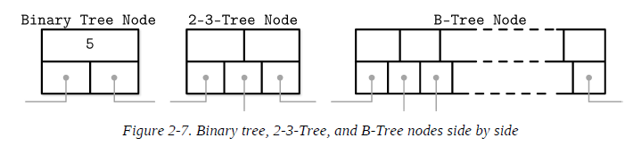
In most of the literature, binary tree nodes are drawn as circles. Since each node is responsible just for one key and splits the range into two parts, this level of detail is sufficient and intuitive. At the same time, B-Tree nodes are often drawn as rectangles, and pointer blocks are also shown explicitly to highlight the relationship between child nodes and separator keys.

B-Trees are sorted: keys inside the B-Tree nodes are stored in order. Because of that, to locate a searched key, we can use an algorithm like binary search. This also implies that lookups in B-Trees have logarithmic complexity.

Using B-Trees, we can efficiently execute both point and range queries. Point queries, expressed by the equality (=) predicate in most query languages, locate a single item. On the other hand, range queries, expressed by comparison (<, >, ≤, and ≥) predicates, are used to query multiple data items in order.

B-Tree Hierarchy

B-Trees consist of multiple nodes. Each node holds up to N keys and N + 1 pointers to the child nodes. These nodes are logically grouped into three groups:

• Root node

  This has no parents and is the top of the tree.

• Leaf nodes

  These are the bottom layer nodes that have no child nodes.

• Internal nodes

  These are all other nodes, connecting root with leaves. There is usually more than one level of internal nodes.

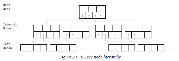
Since B-Trees are a page organization technique (i.e., they are used to organize and navigate fixed-size pages), we often use terms node and page interchangeably.

The relation between the node capacity and the number of keys it actually holds is called occupancy.

B-Trees are characterized by their fanout: the number of keys stored in each node. Higher fanout helps to amortize the cost of structural changes required to keep the tree balanced and to reduce the number of seeks by storing keys and pointers to child nodes in a single block or multiple consecutive blocks. Balancing operations (namely, splits and merges) are triggered when the nodes are full or nearly empty.

B-Trees allow storing values on any level: in root, internal, and leaf nodes. B⁺-Trees store values only in leaf nodes. Internal nodes store only separator keys used to guide the search algorithm to the associated value stored on the leaf level.

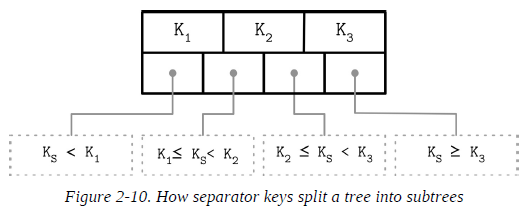
Separator Keys

Keys stored in B-Tree nodes are called index entries, separator keys, or divider cells. They split the tree into subtrees (also called branches or subranges), holding corresponding key ranges. Keys are stored in sorted order to allow binary search. A subtree is found by locating a key and following a corresponding pointer from the higher to the lower level.

The first pointer in the node points to the subtree holding items less than the first key, and the last pointer in the node points to the subtree holding items greater than or equal to the last key. Other pointers are reference subtrees between the two keys: K_i-1 ≤ K_s < K_i , where K is a set of keys, and K_s is a key that belongs to the subtree.

B-Tree Lookup Complexity

To find an item in a B-Tree, we have to perform a single traversal from root to leaf. The objective of this search is to find a searched key or its predecessor. Finding an exact match is used for point queries, updates, and deletions; finding its predecessor is useful for range scans and inserts.

The algorithm starts from the root and performs a binary search, comparing the searched key with the keys stored in the root node until it finds the first separator key that is greater than the searched value. This locates a searched subtree. As soon as we find the subtree, we follow the pointer that corresponds to it and continue the same search process (locate the separator key, follow the pointer) until we reach a target leaf node, where we either find the searched key or conclude it is not present by locating its predecessor.

During the point query, the search is done after finding or failing to find the searched key. During the range scan, iteration starts from the closest found key-value pair and continues by following sibling pointers until the end of the range is reached or the range predicate is exhausted.

B-Tree Node Splits

If the target node to insert or update doesn’t have enough room available, we say that the node has overflowed and has to be split in two to fit the new data. More precisely, the node is split if the following conditions hold:

• For leaf nodes: if the node can hold up to N key-value pairs, and inserting one more key-value pair brings it over its maximum capacity N.

• For nonleaf nodes: if the node can hold up to N + 1 pointers, and inserting one more pointer brings it over its maximum capacity N + 1.

Splits are done by allocating the new node, transferring half the elements from the splitting node to it, and adding its first key and pointer to the parent node. In this case, we say that the key is promoted. The index at which the split is performed is called the split point (also called the midpoint). All elements after the split point (including split point in the case of nonleaf node split) are transferred to the newly created sibling node, and the rest of the elements remain in the splitting node.

If the parent node is full and does not have space available for the promoted key and pointer to the newly created node, it has to be split as well. This operation might propagate recursively all the way to the root.

As soon as the tree reaches its capacity (i.e., split propagates all the way up to the root), we have to split the root node. When the root node is split, a new root, holding a split point key, is allocated. The old root (now holding only half the entries) is demoted to the next level along with its newly created sibling, increasing the tree height by one. The tree height changes when the root node is split and the new root is allocated, or when two nodes are merged to form a new root. On the leaf and internal node levels, the tree only grows horizontally.

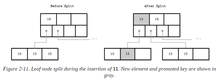
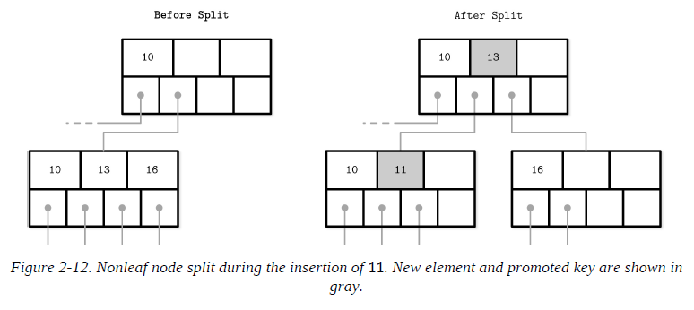
To summarize, node splits are done in four steps:

1. Allocate a new node.

2. Copy half the elements from the splitting node to the new one.

3. Place the new element into the corresponding node.

4. At the parent of the split node, add a separator key and a pointer to the new node.

B-Tree Node Merges

Deletions are done by first locating the target leaf. When the leaf is located, the key and the value associated with it are removed.

If neighboring nodes have too few values (i.e., their occupancy falls under a threshold), the sibling nodes are merged. This situation is called underflow: if two adjacent nodes have a common parent and their contents fit into a single node, their contents should be merged (concatenated); if their contents do not fit into a single node, keys are redistributed between them to restore balance.

• For leaf nodes: if a node can hold up to N key-value pairs, and a combined number of key-value pairs in two neighboring nodes is less than or equal to N.

• For nonleaf nodes: if a node can hold up to N + 1 pointers, and a combined number of pointers in two neighboring nodes is less than or equal to N + 1.

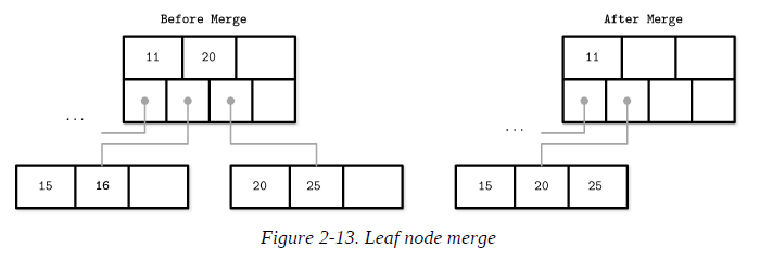
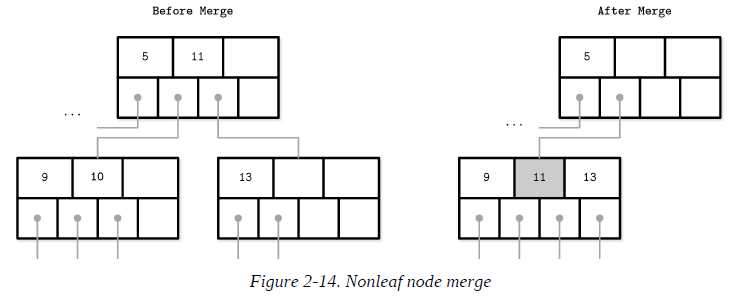
To summarize, node merges are done in three steps, assuming the element is already removed:

1. Copy all elements from the right node to the left one.

2. Remove the right node pointer from the parent (or demote it in the case of a nonleaf merge).

3. Remove the right node.

File Formats

Disks are accessed using system calls. We usually have to specify the offset inside the target file, and then interpret on-disk representation into a form sutable for main memory. To to that, we have to come up with a file format that’s easy to construct, modify, and interpret.

Binary Encoding

Keys and values have a type, such as integer, date, or string and can be represented (serialized to and deserialized from) in their raw binary forms.

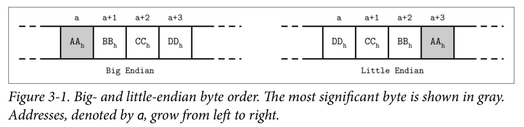
Most numeric data types are represented as fixed-size values. When working with multibyte numeric values, it is important to use the same byte-order (endianness) for both encoding and decoding.

Big-endian

The order starts from the most-significant byte (MSB), followed by the bytes in decreasing significance order. In other words, MSB has the lowest address.

Little-endian

The order starts form the least-significant byte (LSB), followed by the bytes in increasing significance order.

Records consist of primitives like numbers, strings, booleans, and their combinations. However, when transferring data over the network or storing it on disk, we can only use byte sequences. This means that, in order to send or write the record, we have to serialize it (convert it to an interpretable sequence of bytes) and, before we can use it after receiving or reading, we have to deserialize it (translate the sequence of bytes back to the original record).

In binary data formats, we always start with primitives that serve as building blocks for more complex structures. Different numeric types may vary in size. byte value is 8 bits, short is 2 bytes (16bits), int is 4 bytes (32 bits), and long is 8 bytes (64bits).

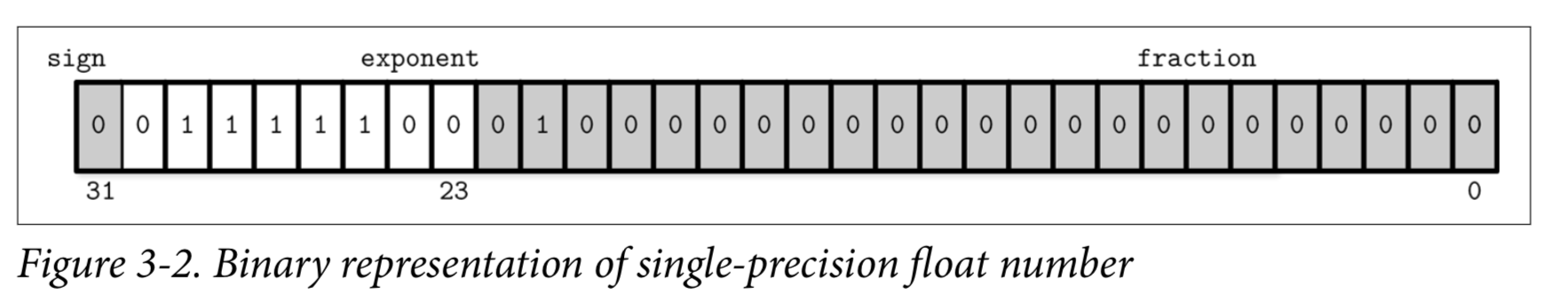
Floating-point numbers (such as float and double) are represented by their sign, fraction, and exponent. The IEEE Standard for Binary Floating-Point Arithmetic (IEEE 754) standard describes widely accepted floating-point number representation.

Strings and other variables-size data types (such as arrays of fixed-size data) can be serialized as a number, representing the length of the array or string, followed by size bytes: the actual data. For strings, this representation is often called UCSD String or Pascal String, named after the popular implementation of the Pascal programming language. We can express it in pseudocode as follows:

String
{
    size uint_16
    data byte[size]
}

An alternative to Pascal strings is null-terminated strings, where the reader consumes the string byte-wise until the end-of-string symbol is reached. The Pascal string approach has several advantages: it allows finding out a length of a string in constant time, instead of iterating through string contents, and a language-specific string can be composed by slicing size bytes from memory and passing the byte array to a string constructor.

Bit-Packed Data: Booleans, Enums, and Flags

Booleans can be represented either by using a single byte, or encoding true and false as 1 and 0 values. Since a boolean has only two values, using an entire byte for its representation is wasteful, and developers often batch boolean values together in groups of eight, each boolean occupying just one bit. We say that every 1 bit is set and every 0 bit is unset or empty.

Enums, short for enumerated types, can be represented as integers and are often used in binary formats and communication protocols.

enum NodeType {
   ROOT,     // 0x00h
   INTERNAL, // 0x01h
   LEAF      // 0x02h
};

Another closely related concept is flags, kind of a combination of packed booleans and enums. Flags can represent nonmutually exclusive named boolean parameters.

Just like packed booleans, flag values can be read and written from the packed value using bitmasks and bitwise operators.

General Principles

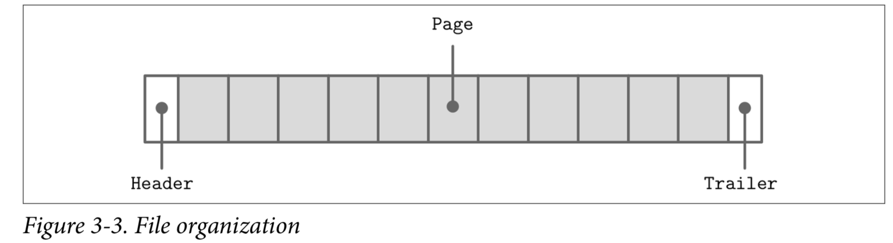
Usually, you start designing a file format by deciding how the addressing is going to be done: whether the file is going to be split into same-sized pages, which are repre‐ sented by a single block or multiple contiguous blocks. Most in-place update storage structures use pages of the same size, since it significantly simplifies read and write access. Append-only storage structures often write data page-wise, too: records are appended one after the other and, as soon as the page fills up in memory, it is flushed on disk.

The file usually starts with a fixed-size header and may end with a fixed-size trailer, which hold auxiliary information that should be accessed quickly or is required for decoding the rest of the file. The rest of the file is split into pages.

Many data stores have a fixed schema, specifying the number, order, and type of fields the table can hold. Having a fixed schema helps to reduce the amount of data stored on disk: instead of repeatedly writing field names, we can use their positional identifiers.

Fixed-size fields:
| (4 bytes) employee_id                |
| (4 bytes) tax_number                 |
| (3 bytes) date                       |
| (1 byte)  gender                     |
| (2 bytes) first_name_length          |
| (2 bytes) last_name_length           |

Variable-size fields:
| (first_name_length bytes) first_name |
| (last_name_length bytes) last_name   |

Database files often consist of multiple parts, with a lookup table aiding navigation and pointing to the start offsets of these parts written either in the file header, trailer, or in the separate file.

Page Structure

Database systems store data records in data and index files. These files are partitioned into fixed-size units called pages, which often have a size of multiple filesystem blocks. Page sizes usually range from 4 to 16 Kb.

Let’s take a look at the example of an on-disk B-Tree node. From a structure perspective, in B-Trees, we distinguish between the leaf nodes that hold keys and data records pairs, and nonleaf nodes that hold keys and pointers to other nodes. Each B-Tree node occupies one page or multiple pages linked together, so in the context of B-Trees the terms node and page (and even block) are often used interchangeably.

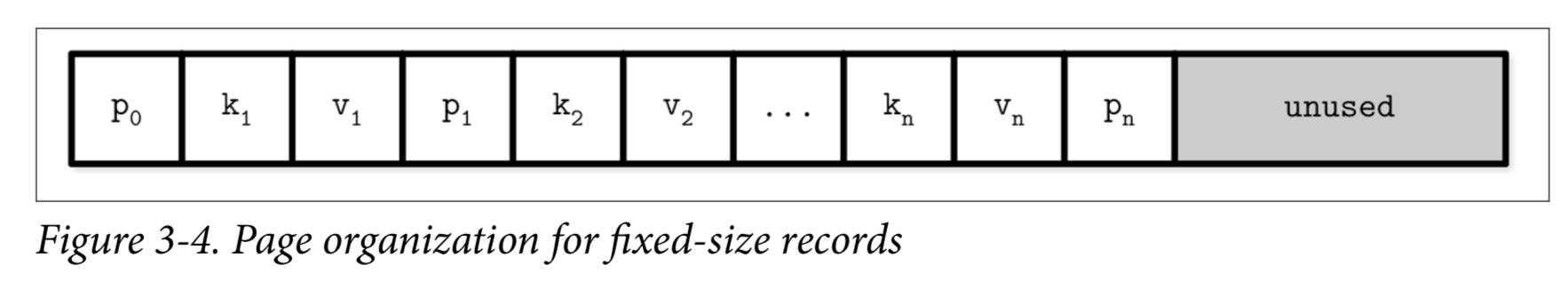
This approach is easy to follow, but has some downsides:

• Appending a key anywhere but the right side requires relocating elements.

• It doesn’t allow managing or accessing variable-size records efficiently and works only for fixed-size data.