Algorithms
An algorithm is any well-defined computational procedure for solving a well-specified computational problem that takes some value, or set of values, as input and produces some value, or set of values, as output.
For example, given the input sequence [31 41 59 26 41 58], a sorting algorithm returns as output [26 31 41 41 58 59]. Such an input sequence is called an instance of the sorting problem.
In general, an instance of a problem consists of the input (satisfying whatever constraints are imposed in the problem statement) needed to compute a solution to the problem.
An algorithm is said to be correct if, for every input instance, it halts with the correct output. An incorrect algorithm might not halt at all on some input instances, or it might halt with an incorrect answer. Contrary to what you might expect, incorrect algorithms can sometimes be useful, if we can control their error rate. Ordinarily, however, we shall be concerned only with correct algorithms.
A data structure is a way to store and organize data in order to facilitate access and modifications. No single data structure works well for all purposes, and so it is important to know the strengths and limitations of several of them.
INSERTION-SORT(A)
1    for j = 2 to A.length
2       key = A[j]
3       // Insert A[j]  into the sorted sequence A[1:j-1].
4       i = j - 1
5       while i > 0 and A[i] > key
6           A[i+1] = A[i]
7           i = i - 1
8       A[i+1] = key
At the start of each iteration of the for loop of lines 1–8, the subarray A[1:j-1] consists of the elements originally in A[1:j-1], but in sorted order, formally called as a loop invariant.
-
Initialization: It is true prior to the first iteration of the loop.
-
Maintenance: If it is true before an iteration of the loop, it remains true before the next iteration.
-
Termination: When the loop terminates, the invariant gives us a useful property that helps show that the algorithm is correct.
Note the similarity to mathematical induction, where to prove that a property holds, you prove a base case and an inductive step until the loop terminates instead of infinitely.
1. Analyzing algorithms
Analyzing an algorithm has come to mean predicting the resources that the algorithm requires, such as memory, communication bandwidth, or computer hardware are of primary concern, but most often it is computational time to be measured.
The time taken by the INSERTION-SORT procedure depends on the size of the input, and how nearly already sorted about two input sequences of the same size: sorting a thousand numbers takes longer than sorting three numbers.
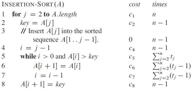
For each j = 2,3, … ,n, where n = A.length, we let tj denote the number of times the while loop test in line 5 is executed for that value of j. When a for or while loop exits in the usual way (i.e., due to the test in the loop header), the test is executed one time more than the loop body. The running time of INSERTION-SORT T(n) on an input of n values is the sum of the products of the cost and times columns.
Even for inputs of a given size, an algorithm’s running time may depend on which input of that size is given.
-
If the array is already sorted, for each
j = 2,3, … ,nandA[i] > keyin line 5,tj = 1and the best-case running time can be expressed asan + bfor constantsaandbthat depend on the statement costsci; it is thus a linear function ofn. -
If the array is in reverse sorted order—that is, in decreasing order—the worst case results. Each element
A[j]must be compared with each element in the entire sorted subarrayA[1:j-1], and sotj = jforj = 2,3, … ,n.The worst-case running time can be expressed as
an2 + bn + cfor constantsa,b, andcthat again depend on the statement costsci; it is thus a quadratic function ofn.
|
The worst-case running time of an algorithm gives us an upper bound on the running time for any input. Knowing it provides a guarantee that the algorithm will never take any longer. It need not to be made some educated guess about the running time and hope that it never gets much worse. |
|
One algorithm is usually considered to be more efficient than another if its worst case running time has a lower order of growth. Due to constant factors and lowerorder terms, an algorithm whose running time has a higher order of growth might take less time for small inputs than an algorithm whose running time has a lower order of growth. |
1.1. Divide-and-conquer algorithms
For insertion sort, it’s used an incremental approach: having sorted the subarray A[1 … j-1], the single element A[j] is inserted into its proper place, yielding the sorted subarray A[1 … j].
Many useful algorithms are recursive in structure: to solve a given problem, they call themselves recursively one or more times to deal with closely related subproblems. These algorithms typically follow a divide-and-conquer approach: they break the problem into several subproblems that are similar to the original problem but smaller in size, solve the subproblems recursively, and then combine these solutions to create a solution to the original problem.
The divide-and-conquer paradigm involves three steps at each level of the recursion:
-
Divide the problem into a number of subproblems that are smaller instances of the same problem.
-
Conquer the subproblems by solving them recursively. If the subproblem sizes are small enough, however, just solve the subproblems in a straightforward manner.
-
Combine the solutions to the subproblems into the solution for the original problem.
The merge sort algorithm closely follows the divide-and-conquer paradigm. Intuitively, it operates as follows.
-
Divide: Divide the n-element sequence to be sorted into two subsequences of n/2 elements each.
-
Conquer: Sort the two subsequences recursively using merge sort.
-
Combine: Merge the two sorted subsequences to produce the sorted answer.
The recursion “bottoms out” when the sequence to be sorted has length 1, in which case there is no work to be done, since every sequence of length 1 is already in sorted order.
The key operation of the merge sort algorithm is the merging of two sorted sequences in the “combine” step.
-
It’s merged by calling an auxiliary procedure
MERGE(A, p, q, r), whereAis an array andp,q, andrare indices into the array such thatp <= q < r. -
The procedure assumes that the subarrays
A[p … q]andA[q + 1 … r]are in sorted order. It merges them to form a single sorted subarray that replaces the current subarrayA[p … r].MERGE(A, p, q, r) // merge the subarrays A[p:q] and A[q+1:r] 1 n1 = q - p + 1 // calculate the length of subarray 2 n2 = r - q 3 let L[1 : n1 + 1] and R[1 : n2 + 1] be new arrays 4 for i = 1 to n1 // copy the subarray A[p:q] to L[1:n1] 5 L[i] = A[p + i - 1] 6 for j = 1 to n2 // copy the subarray A[q + 1: r] to R[1:n2] 7 R[j] = A[q + j] 8 L[n1 + 1] = ∞ // use ∞ as the sentinel value to check whether the subarray is empty 9 R[n2 + 1 = ∞ 10 i = 1 // i is the index of L 11 j = 1 // j is the index of R 12 for k = p to r // k is the index of the loop invariant A[p:r] 13 if L[i] <= R[j] 14 A[k] = L[i] 15 i = i + 1 16 else A[k] = R[j] 17 j = j + 1
-
The procedure
MERGE-SORT(A, p, r)sorts the elements in the subarrayA[p:r]. Ifp >= r, the subarray has at most one element and is therefore already sorted. Otherwise, the divide step simply computes an indexqthat partitionsA[p:r]into two subarrays:A[p:q]andA[q + 1 : r].MERGE-SORT(A, p, r) 1 if p < r 2 q = math.floor[(p + r) / 2] 3 MERGE-SORT(A, p, q) 4 MERGE-SORT(A, q + 1, r) 5 MERGE(A, p, q, r)
Here is the recursion tree that describes the operation of merge sort on the arrayA = [5, 2, 4, 7, 1, 3, 2, 6]. The lengths of the sorted sequences being merged increase as the algorithm progresses from bottom to top.(1, 2, 2, 3, 4, 5, 6, 7) / \ (2, 4, 5, 7) (1, 2, 3, 6) / \ / \ (2, 5) (4, 7) (1, 3) (2, 6) / \ / \ / \ / \ (5) (2) (4) (7) (1) (3) (2) (6)
When an algorithm contains a recursive call to itself, it can be often described its running time by a recurrence equation or recurrence, which describes the overall running time on a problem of size n in terms of the running time on smaller inputs. It can be then used mathematical tools (i.e. master theorem) to solve the recurrence and provide bounds on the performance of the algorithm.
A recurrence for the running time of a divide-and-conquer algorithm falls out from the three steps of the basic paradigm.
-
As before, we let
T(n)be the running time on a problem of sizen. If the problem size is small enough, sayn ⇐ cfor some constantc, the straightforward solution takes constant time, wrote asΘ(1). -
Suppose that our division of the problem yields
asubproblems, each of which is1/bthe size of the original.For merge sort, both
aandbare 2, but we shall see many divide-and-conquer algorithms in which a != b.It takes time
T(n/b)to solve one subproblem of sizen/b, and so it takes timeaT(n/b)to solveaof them. -
If it’s token
D(n)time to divide the problem into subproblems andC(n)time to combine the solutions to the subproblems into the solution to the original problem, the recurrence will beΘ(1)ifn <= c, otherwise,aT(n/b) + D(n) + C(n), that isΘ(nlgn).
// the initial call should be made with mergeSort(a, 0, len(a)), and r is the length of a.
func mergeSort(a []int, p, r int) {
	var q int
	if p < r-1 { // for any subarray that has at least two elements
		q = int((p + r) / 2)
		mergeSort(a, p, q) // sort the subarray a[p:q]
		mergeSort(a, q, r) // sort the subarray a[q:r]
		merge(a, p, q, r)
	}
}

func merge(a []int, p, q, r int) {
	n1 := q - p
	n2 := r - q
	L := make([]int, n1+1)
	R := make([]int, n2+1)
	for i := 0; i < n1; i++ {
		L[i] = a[p+i]
	}
	for i := 0; i < n2; i++ {
		R[i] = a[q+i]
	}
	L[n1] = math.MaxInt // sentinel
	R[n2] = math.MaxInt

	i, j := 0, 0
	for k := p; k < r; k++ {
		if L[i] < R[j] {
			a[k] = L[i]
			i++
		} else {
			a[k] = R[j]
			j++
		}
	}
}
Bubblesort is a popular, but inefficient, sorting algorithm. It works by repeatedly swapping adjacent elements that are out of order.
BUBBLESORT(A)
1  for i = 1 to A.length - 1
2    for j = A.length downto i + 1
3      if A[j]  < A[j - 1]
4 exchange A[j] with A[j - 1]func bubbleSort[T cmp.Ordered](a []T) {
for i := 0; i < len(a)-1; i++ {
for j := len(a) - 1; j > i; j-- {
if a[j] < a[j-1] {
a[j], a[j-1] = a[j-1], a[j]
}
}
fmt.Println(a)
}
}Appendix A: Pseudocode conventions
-
Indentation indicates block structure.
Using indentation instead of conventional indicators of block structure, such as
beginandendstatements, greatly reduces clutter while preserving, or even enhancing, clarity. -
The looping constructs
while,for, andrepeat-untiland theif-elseconditional construct have interpretations similar to those in C, C++, Java, Python, and Pascal.-
After a for loop immediately, the loop counter’s value is the value that first exceeded the for loop bound.
-
We use the keyword to when a for loop increments its loop counter in each iteration, and we use the keyword downto when a for loop decrements its loop counter.
-
When the loop counter changes by an amount greater than 1, the amount of change follows the optional keyword by.
-
-
The symbol
//indicates that the remainder of the line is a comment. -
A multiple assignment of the form
i = j = eassigns to both variablesiandjthe value of expressione; it should be treated as equivalent to the assignmentj = efollowed by the assignmenti = j. -
Variables (such as
i,j, andkey) are local to the given procedure. We shall not use global variables without explicit indication. -
Array elements are accessed by specifying the array name followed by the index (based one instead of zero) in square brackets.
The notation
:is used to indicate a range of values within an array, thus,A[1:j]indicates the subarray ofAconsisting of thejelementsA[1],A[2],…,A[j]. -
Compound data typically is organized into objects, which are composed of attributes.
-
A particular attribute is accessed using the syntax found in many object-oriented programming languages: the object name, followed by a dot, followed by the attribute name.
-
A variable representing an array or object is treated as a pointer to the data representing the array or object.
-
Sometimes, a pointer gived it the special value
NILwill refer to no object at all.
-
-
Parameters are passed to a procedure by value: the called procedure receives its own copy of the parameters, and if it assigns a value to a parameter, the change is not seen by the calling procedure.
When objects are passed, the pointer to the data representing the object is copied, but the object’s attributes are not.
-
A return statement immediately transfers control back to the point of call in the calling procedure.
Most return statements also take a value to pass back to the caller, and multiple values are allowed to be returned in a single return statement.
-
The boolean operators “and” and “or” are short circuiting.
-
The keyword error indicates that an error occurred because conditions were wrong for the procedure to have been called.