TCP/IP: TCP Congestion Control
When a router is forced to discard data because it cannot handle the arriving traffic rate, is called congestion. A router is said to be congested when it is in this state, and even a single connection can drive one or more routers into congestion.
Left unaddressed, congestion can cause the performance of a network to be reduced so badly that it becomes unusable. In the very worst cases, it is said to be in a state of congestion collapse.
To either avoid or at least react effectively to mitigate this situation, each TCP implements congestion control procedures.
Congestion control is a set of behaviors determined by algorithms that each TCP implements in an attempt to prevent the network from being overwhelmed by too large an aggregate offered traffic load.
The basic approach is to have TCP slow down when it has reason to believe the network is about to be congested (or is already so congested that routers are discarding packets).
The challenge is to determine exactly when and how TCP should slow down, and when it can speed up again.
|
In today’s wired networks, packet loss is caused primarily by congestion in routers or switches. With wireless networks, transmission and reception errors become a significant cause of packet loss. Determining whether loss is due to congestion or transmission errors has been an active research topic since the mid-1990s when wireless networks started to attain widespread use. |
A value used to hold the estimate of the network’s available capacity is called the congestion window, written more compactly as simply cwnd.
A sender’s actual (usable) window W is then written as the minimum of the receiver’s advertised window awnd and the congestion window:
W = min(cwnd, awnd)
With this relationship, the TCP sender is not permitted to have more than W unacknowledged packets or bytes outstanding in the network.
The total amount of data a sender has introduced into the network for which it has not yet received an acknowledgment is sometimes called the flight size, which is always less than or equal to W.
In general, W can be maintained in either packet or byte units.
This all seems logical but is far from the whole story.
Because both the state of the network and the state of the receiver change with time, the values of both awnd and cwnd change over time.
In addition, because of the lack of explicit signals, the correct value of cwnd is generally not directly available to the sending TCP. Thus, all of the values W, cwnd, and awnd must be empirically determined and dynamically updated.
In addition, as we said before, we do not want W to be too big or too small—we want it to be set to about the bandwidth-delay product (BDP) of the network path, also called the optimal window size. This is the amount of data that can be stored in the network in transit to the receiver.
Bandwidth-delay product from Wikipedia, the free encyclopedia. [BDP]
In data communications, the bandwidth-delay product is the product of a data link’s capacity (in bits per second) and its round-trip delay time (in seconds). The result, an amount of data measured in bits (or bytes), is equivalent to the maximum amount of data on the network circuit at any given time, i.e., data that has been transmitted but not yet acknowledged. A network with a large bandwidth-delay product is commonly known as a long fat network (shortened to LFN, pronounced "elephan(t)" [RFC1072]).
A high bandwidth-delay product is an important problem case in the design of protocols such as Transmission Control Protocol (TCP) in respect of TCP tuning, because the protocol can only achieve optimum throughput if a sender sends a sufficiently large quantity of data before being required to stop and wait until a confirming message is received from the receiver, acknowledging successful receipt of that data. If the quantity of data sent is insufficient compared with the bandwidth-delay product, then the link is not being kept busy and the protocol is operating below peak efficiency for the link. Protocols that hope to succeed in this respect need carefully designed self-monitoring, self-tuning algorithms. The TCP window scale option may be used to solve this problem caused by insufficient window size, which is limited to 65,535 bytes without scaling.
On the Internet, determining the BDP for a connection can be challenging, given that routes, delay, and the level of statistical multiplexing (i.e., sharing of capacity) change as a function of time.
|
Although handling congestion at the TCP sender is our primary area of interest, work has been done on handling the cases where congestion occurs on the reverse path, because of ACKs. In [RFC5690] a method is introduced to inform a TCP receiver of the ACK ratio it should use (i.e., how many packets it should receive before sending an ACK). |
Definitions in TCP Congestion Control [RFC5681]:
SEGMENT: A segment is ANY TCP/IP data or acknowledgment packet (or both).
SENDER MAXIMUM SEGMENT SIZE (SMSS): The SMSS is the size of the largest segment that the sender can transmit.
This value can be based on the maximum transmission unit of the network, the path MTU discovery [RFC1191, RFC4821] algorithm, RMSS (see next item), or other factors. The size does not include the TCP/IP headers and options.
RECEIVER MAXIMUM SEGMENT SIZE (RMSS): The RMSS is the size of the largest segment the receiver is willing to accept.
This is the value specified in the MSS option sent by the receiver during connection startup. Or, if the MSS option is not used, it is 536 bytes [RFC1122]. The size does not include the TCP/IP headers and options.
FULL-SIZED SEGMENT: A segment that contains the maximum number of data bytes permitted (i.e., a segment containing SMSS bytes of data).
RECEIVER WINDOW (rwnd): The most recently advertised receiver window.
CONGESTION WINDOW (cwnd): A TCP state variable that limits the amount of data a TCP can send.
At any given time, a TCP MUST NOT send data with a sequence number higher than the sum of the highest acknowledged sequence number and the minimum of cwnd and rwnd.
INITIAL WINDOW (IW): The initial window is the size of the sender’s congestion window after the three-way handshake is completed.
LOSS WINDOW (LW): The loss window is the size of the congestion window after a TCP sender detects loss using its retransmission timer.
RESTART WINDOW (RW): The restart window is the size of the congestion window after a TCP restarts transmission after an idle period (if the slow start algorithm is used; see section 4.1 for more discussion).
FLIGHT SIZE: The amount of data that has been sent but not yet cumulatively acknowledged.
DUPLICATE ACKNOWLEDGMENT: An acknowledgment is considered a "duplicate" in the following algorithms when
(a) the receiver of the ACK has outstanding data,
(b) the incoming acknowledgment carries no data,
(c) the SYN and FIN bits are both off,
(d) the acknowledgment number is equal to the greatest acknowledgment received on the given connection (TCP.UNA from [RFC793]) and
(e) the advertised window in the incoming acknowledgment equals the advertised window in the last incoming acknowledgment.
Alternatively, a TCP that utilizes selective acknowledgments (SACKs) [RFC2018, RFC2883] can leverage the SACK information to determine when an incoming ACK is a "duplicate" (e.g., if the ACK contains previously unknown SACK information).
|
1. The Classic Algorithms
When a new TCP connection first starts out, it usually has no idea what the initial value for cwnd should be, as it has no idea how much network capacity is available for it to send its data.
TCP learns the value for awnd with one packet exchange to the receiver, but without any explicit signaling, the only obvious way it has to learn a good value for cwnd is to try sending data at faster and faster rates until it experiences a packet drop (or other congestion indicator).
This could be accomplished by either sending immediately at the maximum rate it can (subject to the value of awnd), or it could start more slowly.
Because of the detrimental effects on the performance of other TCP connections sharing the same network path that could be experienced when starting at full rate, a TCP generally uses one algorithm to avoid starting so fast when it starts up to get to steady state. It uses a different one once it is in steady state.
The operation of TCP congestion control at a sender is driven or clocked by the receipt of ACKs.
If a TCP is operating at steady state (with an appropriate value of cwnd), receipt of an ACK indicates that one or more packets have been removed from the network, and consequently that an opportunity to send more has arisen.
Following this line of reasoning, the TCP congestion behavior in steady state attempts to achieve a conservation of packets in the network.
-
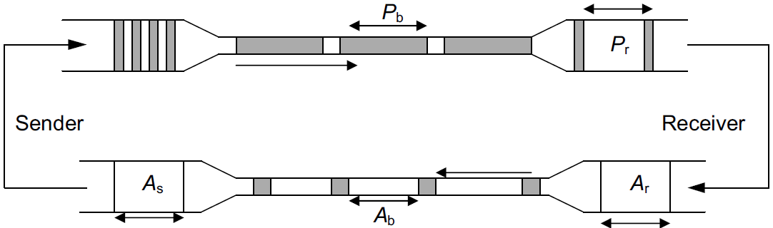
The top funnel holds (larger) data packets traveling along the path from the sender to the receiver.
-
The comparatively narrow width of the funnel depicts how packets are stretched out in time as they travel through a relatively slow link.
-
The ends of the funnels (at sender and receiver) show the queues where packets are held before or after they travel along the path.
-
The bottom funnel holds the ACKs sent by the receiver back to the sender that correspond to the data packets in the top funnel.
-
When operating efficiently at steady state, there are no bunches of packets in the top or bottom funnels.
-
In addition, there is no significant extra space between packets in the top funnel.
-
Note that an arrival of an ACK at the sender liberates another data packet to be sent into the top funnel, and that this happens at just the right time (i.e., when the network is able to accept another packet).
-
This relationship is sometimes called self-clocking, because the arrival of an ACK, called the ACK clock, triggers the system to take the action of sending another packet.
1.1. Slow Start
The slow start algorithm is executed when a new TCP connection is created or when a loss has been detected due to a retransmission timeout (RTO). It may also be invoked after a sending TCP has gone idle for some time.
-
The purpose of slow start is to help TCP find a value for cwnd before probing for more available bandwidth using congestion avoidance and to establish the ACK clock.
-
Typically, a TCP begins a new connection in slow start, eventually drops a packet, and then settles into steady-state operation using the congestion avoidance algorithm.
To quote from [RFC5681]:
Beginning transmission into a network with unknown conditions requires TCP to slowly probe the network to determine the available capacity, in order to avoid congesting the network with an inappropriately large burst of data. The slow start algorithm is used for this purpose at the beginning of a transfer, or after repairing loss detected by the retransmission timer.
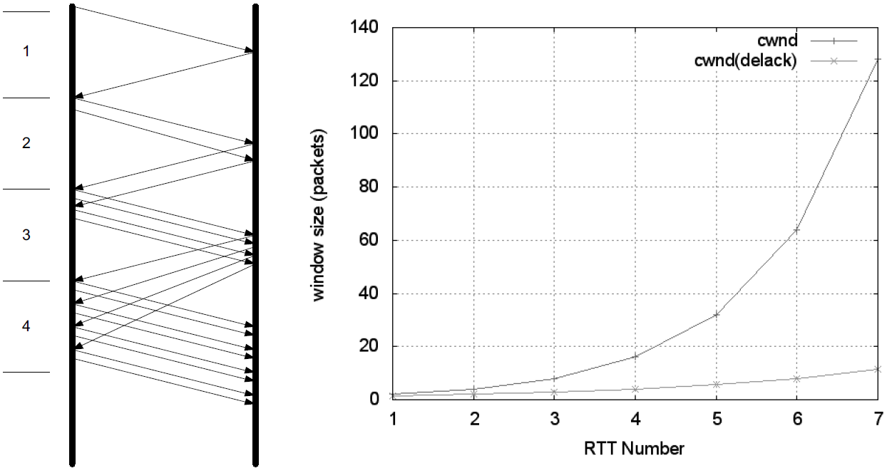
TCP begins in slow start by sending a certain number of segments (after the SYN exchange), called the initial window (IW).
The value of IW was originally one SMSS, although with [RFC5681] it is allowed to be larger.
| Note that in most cases SMSS is equal to the smaller of the receiver’s MSS and the path MTU (less header sizes). |
Assuming no packets are lost and each packet causes an ACK to be sent in response, an ACK is returned for the first segment, allowing the sending TCP to send another segment.
However, slow start operates by incrementing cwnd by min(N, SMSS) for each good ACK received, where N is the number of previously unacknowledged bytes ACKed by the received good ACK.
| A good ACK is one that returns a higher ACK number than has been seen so far. |
Thus, after one segment is ACKed, the cwnd value is ordinarily increased to 2, and two segments are sent. If each of those causes new good ACKs to be returned, 2 increases to 4, 4 to 8, and so on.
-
In general, assuming no loss and an ACK for every packet, the value of W after k round-trip exchanges is W = 2k.
-
Rewriting, we can say that k = log2W RTTs are required to reach an operating window of W.
This growth seems quite fast (increasing as an exponential function) but is still slower than what TCP would do if it were allowed to send immediately a window of packets equal in size to the receiver’s advertised window. Recall that W is still never allowed to exceed awnd.
Eventually, cwnd (and thus W) could become so large that the corresponding window of packets sent overwhelms the network (recall that TCP’s throughput rate is proportional to W/RTT).
-
When this happens, cwnd is reduced substantially (to half of its former value).
-
In addition, this is the point at which TCP switches from operating in slow start to operating in congestion avoidance.
The switch point is determined by the relationship between cwnd and a value called the slow start threshold (or ssthresh).
1.2. Congestion Avoidance
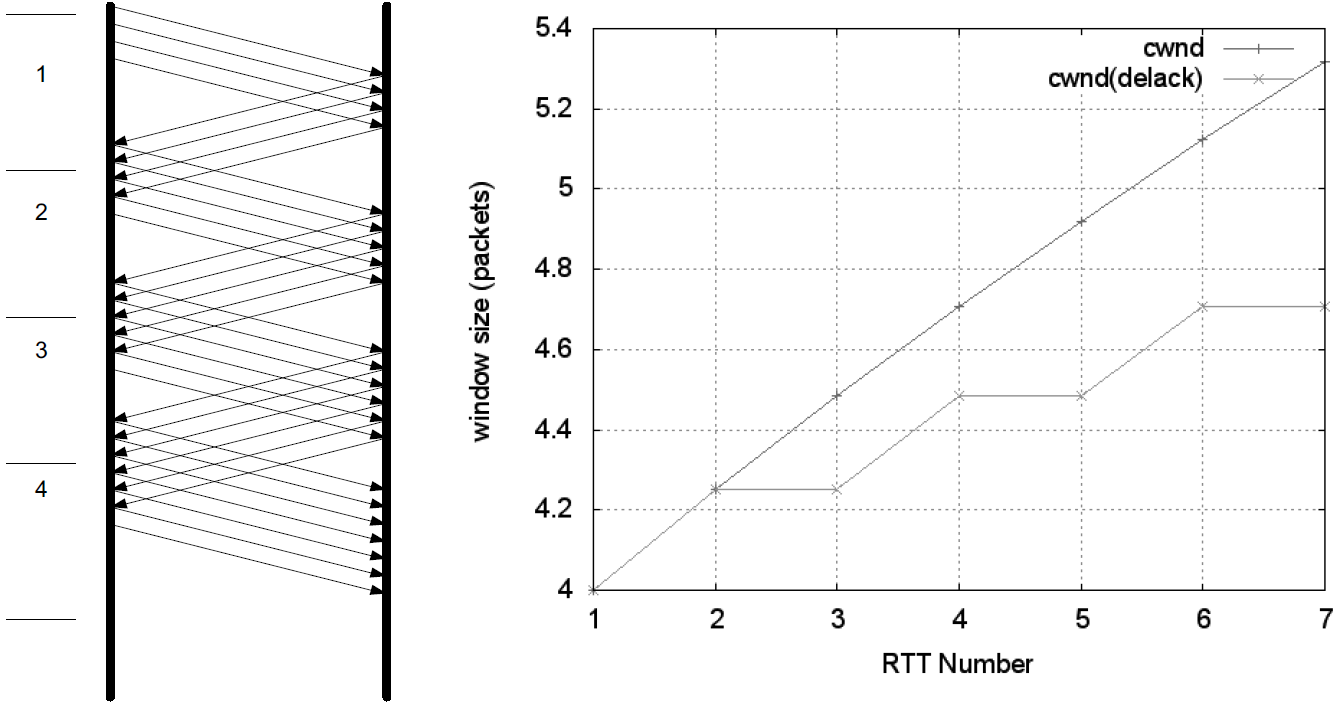
To find additional capacity that may become available, but to not do so too aggressively, TCP implements the congestion avoidance algorithm.
Once ssthresh is established and cwnd is at least at this level, a TCP runs the congestion avoidance algorithm, which seeks additional capacity by increasing cwnd by approximately one segment for each window’s worth of data that is moved from sender to receiver successfully.
This provides a much slower growth rate than slow start: approximately linear in terms of time, as opposed to slow start’s exponential growth.
More precisely, cwnd is usually updated as follows for each received nonduplicate ACK:
cwndt+1 = cwndt + SMSS * SMSS/cwndt
Looking at this relationship briefly, assume cwnd0 = k*SMSS bytes were sent into the network in k segments. After the first ACK arrives, cwnd is updated to be larger by a factor of (1/k):
cwnd1 = cwnd0 + SMSS * SMSS/cwnd0

= k*SMSS + SMSS * (SMSS/(k*SMSS))

= k*SMSS + (1/k) * SMSS

= (k + (1/k))*SMSS

= cwnd0 + (1/k)*SMSS
Because the value of cwnd grows slightly with each new ACK arrival, and this value is in the denominator of the expression in the first equation above, the overall growth rate of cwnd is slightly sublinear.
The assumption of the algorithm is that packet loss caused by bit errors is very small (much less than 1%), and therefore the loss of a packet signals congestion somewhere in the network between the source and destination.
-
If this assumption is false, which it sometimes is for wireless networks, TCP slows down even when no congestion is present.
-
In addition, many RTTs may be required for the value of cwnd to grow large, which is required for efficient use of networks with high capacity.
1.3. Selecting between Slow Start and Congestion Avoidance
In normal operations, a TCP connection is always running either the slow start or the congestion avoidance procedure, but never the two simultaneously.
-
When cwnd < ssthresh, slow start is used, and when cwnd > ssthresh, congestion avoidance is used.
-
When they are equal, either can be used.
The initial value of ssthresh may be set arbitrarily high (e.g., to awnd or higher), which causes TCP to always start with slow start. When a retransmission occurs, caused by either a retransmission timeout or the execution of fast retransmit, ssthresh is updated as follows:
ssthresh = max(flight size/2, 2*SMSS)
1.4. Tahoe, Reno, and Fast Recovery
The slow start and congestion avoidance constitute the first congestion control algorithms which were introduced in the late 1980s with the 4.2 release of UC Berkeley’s version of UNIX, called the Berkeley Software Distribution, or BSD UNIX.
The 4.2 release of BSD (called Tahoe) included a version of TCP that started connections in slow start, and if a packet was lost, detected by either a timeout or the fast retransmit procedure, the slow start algorithm was reinitiated.
Tahoe was implemented by simply reducing cwnd to its starting value (1 SMSS at that time) upon any loss, forcing the connection to slow start until cwnd grew to the value ssthresh.
One problem with this approach is that for large BDP paths, this can cause the connection to significantly underutilize the available bandwidth while the sending TCP goes through slow start to get back to the point at which it was operating before the packet loss.
To address this problem, the reinitiation of slow start on any packet loss was reconsidered.
-
Ultimately, if packet loss is detected by duplicate ACKs (invoking fast retransmit), cwnd is instead reset to the last value of ssthresh instead of only 1 SMSS.
-
Slow start is still initiated on a timeout, which is generally the case for most TCP variants.
-
This approach allows the TCP to slow down to half of its previous rate without reverting to slow start.
In exploring the issue of large BDP paths further and thinking back to the conservation of packets principle mentioned before, it has been observed that any ACKs that are received, even while recovering after a loss, still represent opportunities to inject new packets into the network.
-
This became the basis of the fast recovery procedure, which was released in conjunction with the popular 4.3 BSD Reno version of BSD UNIX.
-
Fast recovery allows cwnd to (temporarily) grow by 1 SMSS for each ACK received while recovering.
-
The congestion window is therefore inflated for a period of time, allowing an additional new packet to be sent for each ACK received, until a good ACK is seen.
-
Any nonduplicate (good) ACK causes TCP to exit recovery and reduces the congestion back to its pre-inflated value.
TCP Reno became very popular and ultimately the basis for what might reasonably be called "standard TCP".
1.5. Standard TCP
To summarize the combined algorithm from [RFC5681], TCP begins a connection in slow start (cwnd = IW) with a large value of ssthresh, generally at least the value of awnd.
Upon receiving a good ACK (one that acknowledges new data), TCP updates the value of cwnd as follows:
cwnd += SMSS         (if cwnd < ssthresh)        Slow start
cwnd += SMSS*SMSS/cwnd         (if cwnd > ssthresh)        Congestion avoidance
When fast retransmit is invoked because of receipt of a third duplicate ACK (or other signal, if conventional fast retransmit initiation is not used), the following actions are performed:
-
ssthresh is updated to no more than the value given in equation ssthresh = max(flight size/2, 2*SMSS).
-
The fast retransmit algorithm is performed, and cwnd is set to (ssthresh + 3*SMSS).
-
cwnd is temporarily increased by SMSS for each duplicate ACK received.
-
When a good ACK is received, cwnd is reset back to ssthresh.
-
The actions in steps 2 and 3 constitute fast recovery.
-
Step 2 first adjusts cwnd, which usually causes it to be reduced to half of its former value, and then temporarily inflates it to take into account the fact that the receipt of each duplicate ACK indicates that some packet has left the network (and thus should permit another to be inserted).
This step is also where multiplicative decrease occurs, as cwnd is ordinarily multiplied by some value (0.5 here) to form its new value.
-
Step 3 continues the inflation process, allowing the sender to send additional packets (assuming awnd is not exceeded).
-
In step 4, the TCP is assumed to have recovered, so the temporary inflation is removed (and so this step is sometimes called deflation).
Slow start is always used in two cases: when a new connection is started, and when a retransmission timeout occurs.
-
It can also be invoked when a sender has been idle for a relatively long time or there is some other reason to suspect that cwnd may not accurately reflect the current network congestion state.
In this case, the initial value of cwnd is set to the restart window (RW).
In [RFC5681], the recommended value of RW = min(IW, cwnd).
-
Other than this case, when slow start is invoked, cwnd is set to IW.
2. Evolution of the Standard Algorithms
The classic and standard TCP algorithms made a tremendous contribution to the operation of TCP, essentially addressing the major problem of Internet congestion collapse.
|
The problem of Internet congestion collapse was a serious concern during the years 1986–1988. In October 1986 the NSFNET backbone, an important component of the early Internet, had been observed to operate with an effective capacity some 1000 times less than it should have (called the "NSFNET meltdown"). The primary reason for the problem was aggressive retransmissions during times of loss without any controls. This behavior drove the network into a persistently congested state where packet loss was massive (causing more retransmissions) and throughput was low. Adoption of the classic congestion control algorithms effectively eliminated this problem. |
2.1. NewReno
One problem with fast recovery is that when multiple packets are dropped in a window of data, once one packet is recovered (i.e., successfully delivered and ACKed), a good ACK can be received at the sender that causes the temporary window inflation in fast recovery to be erased before all the packets that were lost have been retransmitted.
| ACKs that trigger this behavior are called partial ACKs (ACKs that cover previously unacknowledged data, but not all the data outstanding when loss was detected). |
A Reno TCP reacting to a partial ACK by reducing its inflated congestion window can go idle until a retransmission timer fires.
-
To understand why this happens, recall that (non-SACK) TCP depends on the signal of three (or dupthresh) duplicate ACKs to trigger its fast retransmit procedure.
-
If there are not enough packets in the network, it is not possible to trigger this procedure on packet loss, ultimately leading to the expiration of the retransmission timer and invocation of the slow start procedure, which drastically impacts TCP throughput performance.
To address this problem with Reno, a modification called NewReno [RFC3782] has been developed.
-
This procedure modifies fast recovery by keeping track of the highest sequence number from the last transmitted window of data (the recovery point).
-
Only when an ACK with an ACK number at least as large as the recovery point is received is the inflation of fast recovery removed.
-
This allows a TCP to continue sending one segment for each ACK it receives while recovering and reduces the occurrence of retransmission timeouts, especially when multiple packets are dropped in a single window of data.
NewReno is a popular variant of modern TCPs—it does not suffer from the problems of the original fast recovery and is significantly less complicated to implement than SACKs.
With SACKs, however, a TCP can perform better than NewReno when multiple packets are lost in a window of data, but doing this requires careful attention to the congestion control procedures.
2.2. TCP Congestion Control with SACK
With SACK TCP, the sender can be informed of multiple missing segments and would theoretically be able to send them all immediately because they would all be in the valid window.
However, this might involve sending too much data into the network at once, thereby compromising the congestion control.
The following issue arises with SACK TCP: using only cwnd as a bound on the sender’s sliding window to indicate how many (and which) packets to send during recovery periods is not sufficient.
Instead, the selection of which packets to send needs to be decoupled from the choice of when to send them.
One way to implement this decoupling is to have a TCP keep track of how much data it has injected into the network separately from the maintenance of the window.
-
In [RFC3517] this is called the pipe variable, an estimate of the flight size.
Importantly, the pipe variable counts bytes (or packets, depending on the implementation) of transmissions and retransmissions, provided they are not known to be lost.
-
Assuming a large value of awnd, a SACK TCP is permitted to send a segment anytime the following relationship holds true: cwnd - pipe ≥ SMSS.
In other words, cwnd is still used to place a limit on the amount of data that can be outstanding in the network, but the amount of data estimated to be in the network is accounted for separately from the window itself.
2.3. Forward Acknowledgment (FACK) and Rate Halving
References
-
[ASA00] A. Aggarwal, S. Savage, and T. Anderson, "Understanding the Performance of TCP Pacing", Proc. INFOCOM, Mar. 2004.
-
[TCPIPV1] Kevin Fall, W. Stevens TCP/IP Illustrated: The Protocols, Volume 1. 2nd edition, Addison-Wesley Professional, 2011
-
[RFC1072] V. Jacobson, R. Braden, TCP Extensions for Long-Delay Paths, Internet RFC 1072, Oct. 1988, See https://www.rfc-editor.org/rfc/rfc1072
-
[RFC5681] M. Allman, V. Paxson, E. Blanton, TCP Congestion Control, Internet RFC 5681, Sept. 2009, See https://www.rfc-editor.org/rfc/rfc5681
-
[RFC3782] S. Floyd, T. Henderson, and A. Gurtov, The NewReno Modification to TCP’s Fast Recovery Algorithm, Internet RFC 3782, Apr. 2004, See https://www.rfc-editor.org/rfc/rfc3782
-
[RFC3517]] E. Blanton, M. Allman, K. Fall, and L. Wang, A Conservative Selective Acknowledgment (SACK)-Based Loss Recovery Algorithm for TCP, Internet RFC 3517, Apr. 2003, See https://www.rfc-editor.org/rfc/rfc3517